Academic stock data

Background

If you read this post, you will know I am collecting accounting and fundamental data for US stocks via the SEC EDGAR database. Price and other reference type data is also collected, and you can read about it here. The storage format is a PostgreSQL database.

The SEC data referred to above starts in 2009, and the coverage in the earlier years is patchy. This lack of data is an issue.

Why is that? I am using this data to model how a stocks characteristics (prior returns, valuation, quality, etc) influence its future returns. In doing that I am open to the possibility (it might be more accurate to say I expect) that the relationships between characteristics and returns change over time. Furthermore, it may be that these relationships change based on prevailing macroeconomic factors such as interest rates or growth, or market conditions like volatility. A hypothesis might be that high quality stocks outperform in an economic downturn. Or, stocks with strong prior returns only continue to outperform when volatility is low. Here’s the crutch. There is only one market downturn since 2009. There are limited volatility episodes, the period leading up to the financial crisis is omitted. This is an issue. Estimating a model based on an (expected) recurring phenomena requires as many occurrences of that phenomena as possible, especially when the data is noisy. The more data, the more robust the results.

That’s were the new data I have found comes in.

Data

Obviously it would be great if I had data going back to the early 1990’s covering a significant universe of stocks, the top 1,000 by market capitalisation for example. Sourcing that type of data however is not really feasible for a retail investor / hobbyist. The cost is prohibitive.

If you are in an academic environment the WRDS or CRISP databases are an option. This is where most of the research papers source data. This is also the source from which the well known Fama/French factors are derived.

Fortunately a couple of researchers have decided to make their work available. The website Open Source Asset Pricing “provides test asset returns and signals replicated from the academic asset pricing literature”. It supports the paper by Chen and Zimmerman [1].

The researchers responsible for “Empirical Asset Pricing via Machine Learning” [2] have published the underlying data for that paper on Dacheng Xiu’s website.

Data load

The datasets referred to above are exposed in zipped csv format, which I downloaded locally to my machine. The initial intention was to use the psql copy command to load each of these into Postgres in a single function call for each file. That didn’t work out. I came up against the issues outlined here and here, whereby older versions of Postgres inadvertantly apply a size limit on the file that can be uploaded. Not a big deal, the data just had to be split into smaller portions as detailed in the code below.

This R script reads data into a data frame using data.table, converts the text formatted date into a date type, breaks the data into smaller chunks, saves these to a temporary CSV file, and then loads that file to Postgres calling the psql copy command. Calling the psql command is done via the R system function.

This process worked well, something like 5 million rows and circa 100 columns was inserted into the Postgres daabase in a couple of minutes.

# Libraries
library(data.table)
library(lubridate)

# Load data
 
# Date stamp V1
# https://www.openassetpricing.com/data/
# Convert integer to date & convert to prior month end (datashare.csv >> 'osap' table)
d <- fread("C:/Users/brent/Documents/VS_Code/postgres/postgres/reference/datashare.csv")
d[, date_stamp := strptime(DATE, format="%Y%m%d")]
d[, date_stamp := as.Date(floor_date(date_stamp, "month") - 1)]

# Date stamp V2
# https://dachxiu.chicagobooth.edu/download/datashare.zip
# Convert integer to date & make month end (signed_predictors_dl_wide.csv >> 'eapvml' table)
d <- fread("C:/Users/brent/Documents/VS_Code/postgres/postgres/reference/signed_predictors_dl_wide.csv")
d[, date_stamp := as.Date(paste0(as.character(yyyymm), '01'), format='%Y%m%d')]
d[, date_stamp := date_stamp %m+% months(1) - 1]

# Connect to stock_master db
library(DBI)
library(RPostgres)
library(jsonlite)

config <- jsonlite::read_json('C:/Users/brent/Documents/VS_Code/postgres/postgres/config.json')

con <- DBI::dbConnect(
  RPostgres::Postgres(),
  host      = 'localhost',
  port      = '5432',
  dbname    = 'stock_master',
  user      = 'postgres',
  password  = config$pg_password
)

# Create table schema with sample of data
db_write <- as.data.frame(d[permno == 14593, ])
dbWriteTable(con, Id(schema = "reference", table = "osap"), db_write)
dbSendQuery(conn = con, statement = "delete from reference.osap")

# psql copy command
# https://stackoverflow.com/questions/62225835/fastest-way-to-upload-data-via-r-to-postgressql-12
URI <- sprintf("postgresql://%s:%s@%s:%s/%s", "postgres", config$pg_password, "localhost", "5432", "stock_master")
n <- 100000
w <- floor(nrow(d) / n)
r <- nrow(d) %% (n * w)

for (i in 1:(w+1)) {
  if (i == 1) {
    s <- 1
    e <- n
  } else if (i <= w) {
    s <- s + n
    e <- e + n
  } else {
    s <- s + n
    e <- e + r  
  }
  
  print(paste0(s, " to ", e))
  rng <- s:e
  fwrite(d[rng, ], "temp.csv")
  
  system(
    sprintf(
      "psql -U postgres -c \"\\copy %s from %s delimiter ',' csv header\" %s",
      "reference.osap", 
      sQuote("temp.csv", FALSE), 
      URI
    )
  )
}

DBI::dbDisconnect(con)

Analysis

Let’s take a look at the data we have loaded. The plot below counts the number of stocks returned by date. This is using the ‘Empirical Asset Pricing via Machine Learning’ dataset.

-- Result assigned to object "eapvml"
select permno, date_stamp, mvel1, mom1m from reference.eapvml

# Libraries
library(data.table)
setDT(eapvml)

# Plot number of stocks over time
library(ggplot2)

# Custom theme
cstm_theme1 <- theme_minimal() +
  theme(
    legend.title = element_blank(),
    legend.position = c(0.9,0.9),
    legend.background = element_blank(),
    legend.key = element_blank(),
    plot.caption = element_text(size = 8, color = "grey55", face = 'italic'), 
    axis.title.y = element_text(size = 8, color = "darkslategrey"),
    axis.title.x = element_text(size = 8, color = "darkslategrey"),
    axis.text.y = element_text(size = 7, color = "darkslategrey"),
    axis.text.x = element_text(size = 7, color = "darkslategrey")
    )

ggplot(data=eapvml[, .(stocks_unq = length(unique(permno)), stocks_n = .N), by = date_stamp], 
       aes(x=date_stamp, y=stocks_n, group=1)) +
  geom_line() +
  labs(
    title = "Count of unique stocks",
    subtitle = "Data supporting 'Empirical Asset Pricing via Machine Learning'",
    caption = "Source: https://dachxiu.chicagobooth.edu/download/datashare.zip",
    x = '',
    y = ''
  ) +
  cstm_theme1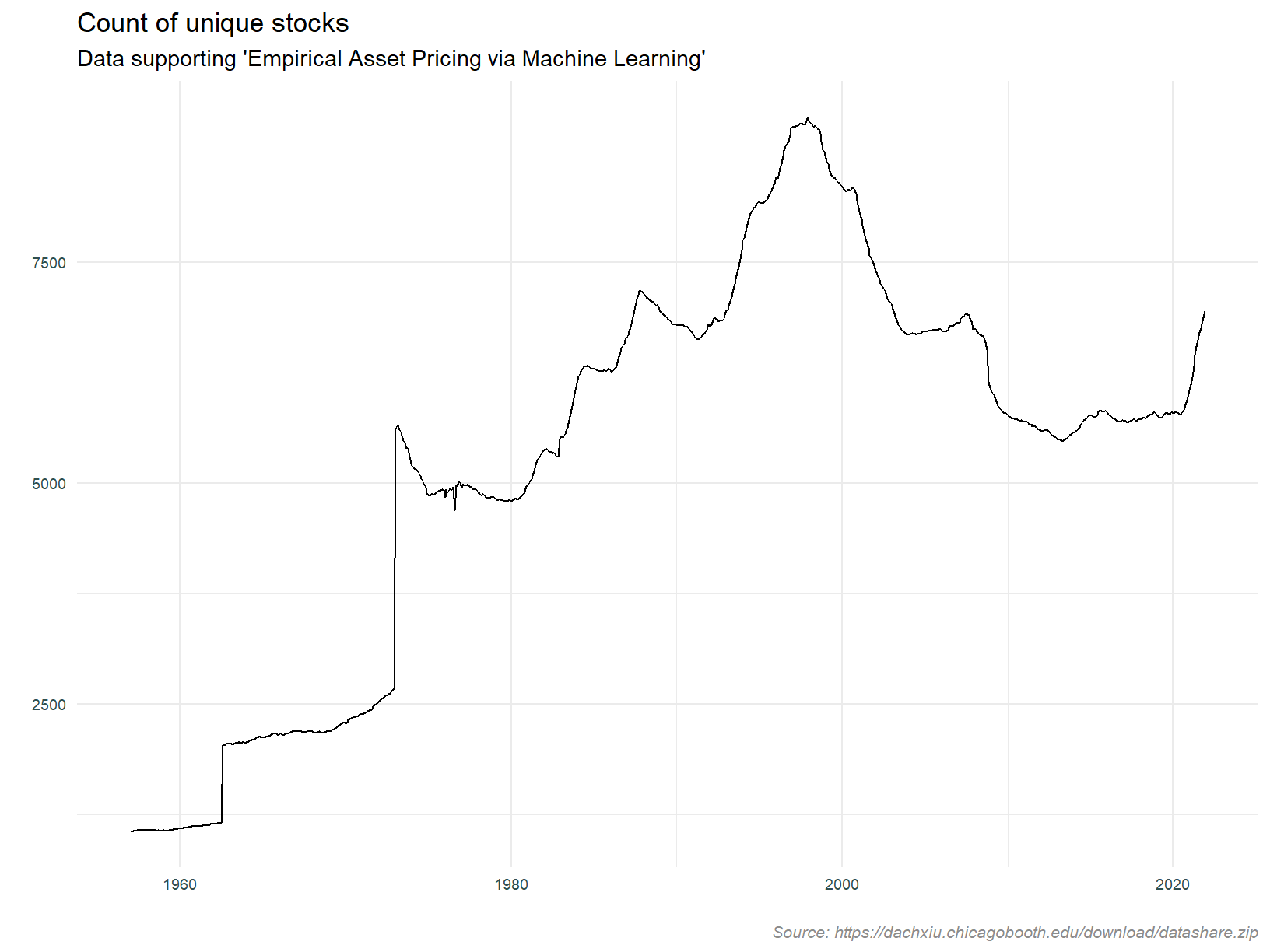

Our data set has roughly 2,000 stocks per month until the mid 1970’s, thereafter they count per month shoots up to circa 5,000, rising to over 8,000 in the 1990’s. This coincides with the tech bubble, as does the decline after bursting of said bubble in 2000. Stocks per monthly increase after 2020, and I speculate that this is due to the SPAC phenomenon. The cause of the drastic increase in the mid 1970’s is not apparent. On that basis, it is prudent to limit analysis to after 1975.

Next, we check that the return attributes in the academic data matches those independently collected from price data. The academic data has an attribute named mom1m which is the monthly arithmetic returns. We can also calculate returns from the change in market capitalisation, mvel1¹.

We need a specific stock to perform this comparison and that is where another issues raises it’s head. Individual stocks in the academic data are identified by their permno.

“PERMNO is a unique permanent security identification number assigned by CRSP to each security. Unlike the CUSIP, Ticker Symbol, and Company Name, the PERMNO neither changes during an issue’s trading history, nor is it reassigned after an issue ceases trading.”

Stocks in the Postgres database are identified by ticker or CIK (Central Index Key). At this point I do not have a mapping between the PERMNO and these two identifiers. AAPL has been the largest stock by market capitalisation over the last few years. Lets find the permno for AAPL, filtering for the largest value of the attribute mvel1, the market value of equity.

select date_stamp, permno from reference.eapvml
where date_stamp = (select max(date_stamp) from reference.eapvml)
and mvel1 = (select max(mvel1) from reference.eapvml)

OK, lets get the price and return data for AAPL, and join it to the return data from our new dataset where the permno is 14593. We will then check for correlation between these returns, if they do indeed represent the same stock, the correlations should be close to one.

-- Result assigned to object "stock_master_aapl"
select 
symbol
,date_stamp
,rtn_ari_1m 
from access_layer.return_attributes
where date_stamp between '2015-01-31'::date and '2021-12-31'::date 
and symbol = 'AAPL'
order by 1,2

setDT(stock_master_aapl)
setorder(eapvml, permno, date_stamp)
eapvml_aapl <- eapvml[permno == 14593][, rtn_ari_1m_ea := (mvel1 - shift(mvel1, 1)) / shift(mvel1, 1)]
cor_data <- eapvml_aapl[stock_master_aapl, on = c("date_stamp"), nomatch = 0][ , .(mom1m, rtn_ari_1m_ea, rtn_ari_1m)]

library(PerformanceAnalytics)
chart.Correlation(cor_data, histogram=TRUE, pch=1)

Well I think we have a match! In the plot above the largest digits are the correlations. mom1m is the precalculated one month return, rtn_ari_1m_ea is the return derived from changes in market capitalization. Both of these come from the new academic data set. rtn_ari_1m is the return calculated from independently collected price data (i.e. that which already exists in the stock market database).

I would put money on permno 14953 being the identifier for Apple².

Lastly, lets look at the turnover of portfolios defined as the top 50, 100, 500 and 1,000 stocks by market capitalisation. We will assess turnover every year. The expectation is that turnover will be higher for the smaller portfolios since it is easier for a stock to move into or out of a smaller group³.

If we see anything untoward here it may be an indicator of data quality issues.

# Function for measuring portfolio turnover
turnover <- function(df, top_n) {
  
  unq_dates   <- sort(unique(df$date_stamp))
  start_dates <- shift(unq_dates)[-1]
  end_dates   <- unq_dates[-1]
  dat         <- Sys.Date()[0]
  res         <- list()
  
  for (i in 1:length(end_dates)) {
    s    <- df[date_stamp == start_dates[i] & mkt_cap_rank %in% 1:top_n, symbol]
    e    <- df[date_stamp == end_dates[i] & mkt_cap_rank %in% 1:top_n, symbol]
    resi <- length(setdiff(s, e)) / length(s)
    dat  <- append(dat, end_dates[i])
    res  <- append(res, resi)
  }
  
  return(data.frame(date_stamp = dat, turnover = unlist(res)))
}

# Create data frame with december dates including rank by mkt cap
turnoverd <- eapvml[month(date_stamp) == 12 & date_stamp > as.Date('1980-12-31'), .(date_stamp, permno, mvel1)][, mkt_cap_rank := frankv(mvel1, order = -1), by = date_stamp]
setnames(turnoverd, old = "permno", new = "symbol")

# Call turnover function
t50 <- turnover(turnoverd, top_n = 50)
t50$top_n <- 50
t100 <- turnover(turnoverd, top_n = 100)
t100$top_n <- 100
t500 <- turnover(turnoverd, top_n = 500)
t500$top_n <- 500
t1000 <- turnover(turnoverd, top_n = 1000)
t1000$top_n <- 1000
t <- rbind(t50, t100, t500, t1000)

ggplot(data=t, aes(x=date_stamp, y=turnover, group=1)) +
  geom_line() +
  facet_wrap(vars(top_n)) +
  labs(
    title = "Portfolio turnover",
    subtitle = "Data supporting 'Empirical Asset Pricing via Machine Learning'",
    caption = "Source: https://dachxiu.chicagobooth.edu/download/datashare.zip",
    x = '',
    y = ''
  ) +
  cstm_theme1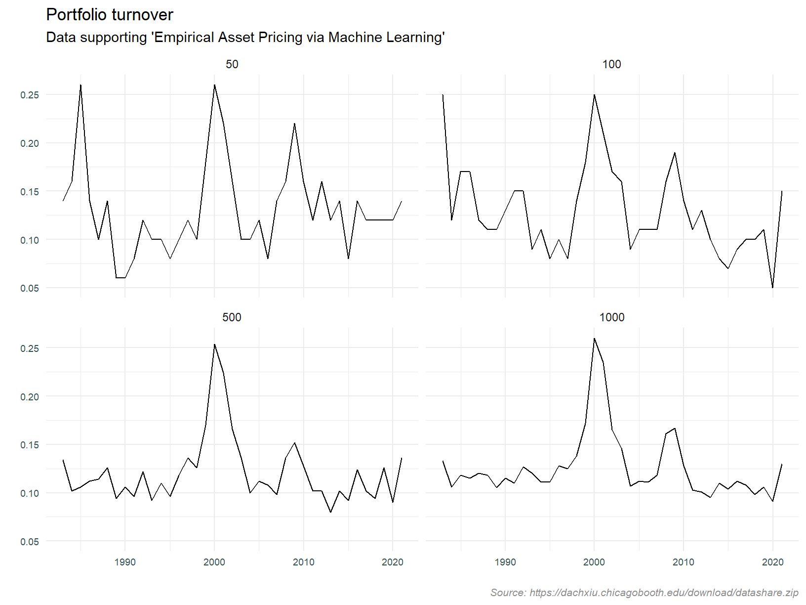

What are we seeing here?

• Turnover is less volatile as the group is larger
  
• Average turnover is higher for the smaller large cap groups
  
• There was a spike in turnover when the tech bubble burst

All in all, the analysis of portfolio turnover doesn’t raise any red flags.

Conclusion

I’m will continue to interrogate this data and verify some of the fundamental data points exposed in the academic dataset. That will entail back engineering balance sheet and income statement metrics from ratios such as price/book, price/earnings, etcetera (based on what I know thus far, in some cases that will require a second generation back engineering using accounting identities). I will find an overlap between the SEC data in my database and that referred to above and check alignment.

More to come here…

References

[1] Chen A and Zimmerman T, 2021, Open Source Cross-Sectional Asseis identified by the t Pricing, Critical Finance Review 2022. Available at SSRN: https://papers.ssrn.com/sol3/papers.cfm?abstract_id=3604626

[2] Gu S, Kelly B and Xiu D, Empirical Asset Pricing via Machine Learning, The Review of Financial Studies, Volume 33, Issue 5, May 2020, Pages 2223-2273, https://doi.org/10.1093/rfs/hhaa009