“datasets are often highly structured, containing clusters of non-independent observational units that are hierarchical in nature, and Linear Mixed Models allow us to explicitly model the non-independence in such data”
(Harrison et al., 2018) [1]
They allow modeling of data measured on different levels at the same time - for instance students nested within classes and schools - thus taking complex dependency structures into account
(Burkner, 2018) [2]
These models inherently regularize estimates towards a central value to an extent that depends on the heterogeneity of the underlying groups.
(Green & Thomas, 2019) [3]
The regularizing aspects of the ‘partial pooling’ inherent in the structure of these models (averaging parameter estimates between in-group and across-subject loadings) help to mitigate the impacts of multiple comparisons by pulling an estimate towards its central tendency to the extent warranted by the between-group variance
(Green & Thomas, 2019) [3]
This post will be an investigation into various types of regression models. The intent is to gain an intuition across a multitude of techniques and the context for this will be assessing stock valuation. A particular focus will be on multi-level models and ensuring robustness in the presence of outliers.
In order to do this we need a model, and I’m going to use the P/B - ROE model. This model relates the ratio of market capitalisation over book value to return on equity. We expect the regression co-efficient on ROE is positive, indicating that holding book value constant, a higher ROE leads to a higher valuation.
Regression techniques to be assessed will cover linear models estimated using ordinary least squares (on a pooled and un-pooled basis), multi-levels models (estimated using both frequentist and Bayesian approaches), and as mentioned above, non-parametric robust technique. Multi-level models will be extended to account for measurement error in predictor variables, a useful technique that Bayesian estimation allows us to implement. We will also model the response with a non-normal link functions, using the Student’s t distribution to account for outlying data points.
As alluded to in the quotes above, the focus will be on multi-level models. Why this particular focus? Multi-level models purport to provide robust results by virtue of partial pooling. Partial pooling results in regularisation of parameter estimates via the sharing of information across groups or clusters of observations. Stocks naturally fall into groups based on industry membership. This makes multi-level models a highly relevant technique in the modeling of stock valuations.
Robust regression techniques also purport to provide robust results (it’s all in the name isn’t it). We will see how these techniques, multi-level parametric and robust non-parametric, compare.
The Theil-Sen regression is a non-parametric robust technique. Theil-Sen has been discussed here, and is a robust technique that works to dampen the impact of outliers. It does so whereby the slope is derived taking the median of many individual slopes, those being fitted to each pair of data points.
Two approaches that have a similar aim, but take different routes to model data. It will be interesting to review the difference in fit between models that pool data and embed an underlying distributional assumption, and those that are non-parametric and use robust techniques.
The code behind this post can be found here.
The data
The data under analysis comprises around 750 individual companies. These companies are grouped into 11 sectors and 40 odd industries. The data is as of June 2021 and comes from the Securites and Exchange Commission via my Stock_master database.
Below are some variables of interest. Our dependent variable is log_pb, the independent variable is roe.
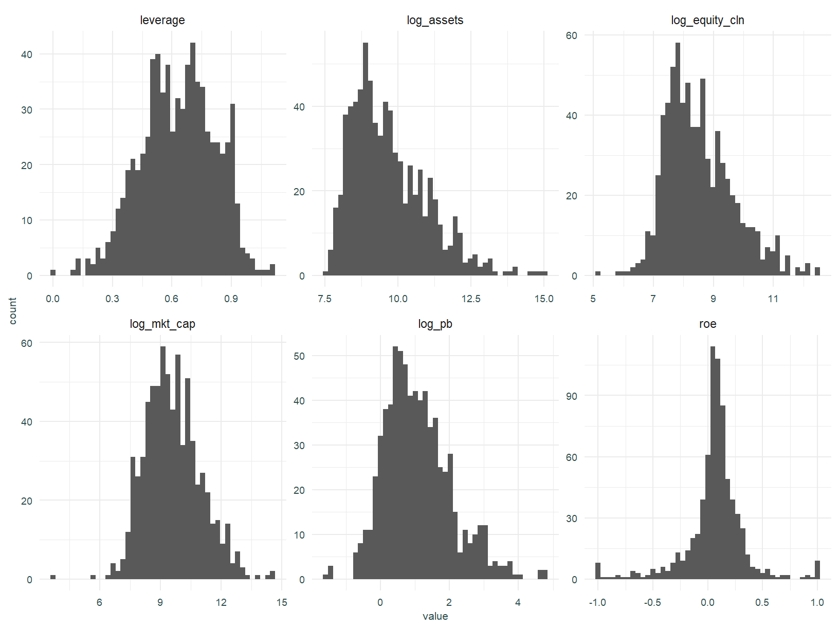
Some definitions, leverage is debt over assets, log_assets is the natural logarithm of total assets, log_equity_cln is the natural logarithm of total equity when equity is positive and the natural logarithm of 10% of assets when equity is negative, and roe is return on equity.
Aggregate analysis
We start applying our model to the full data set, ignoring the underlying sector structure.
The plot below shows the relationship between the log price/book ratio and ROE for all stocks regardless of sector or industry membership. The blue line is the regression line fitted using OLS, the grey line that fitted using the Theil-Sen robust estimator, and magenta is a Generalised Additive Model with a spline smooth.
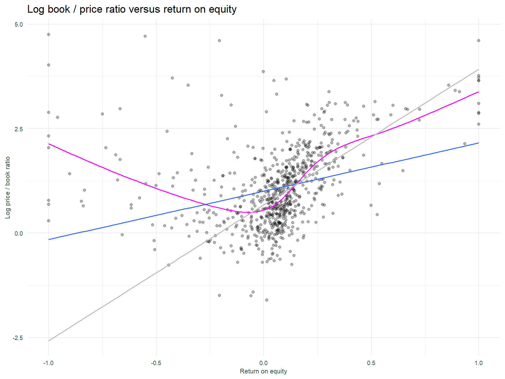
The Theil-Sen regression seems to fit the data better (at least on a rough eyeballing of the plot), fitting the dense cluster of data points more closely. As expected, the slope of the line is positive, indicating all else equal, a higher valuation given higher return on equity.
There is a hint of non-linearity in the relationship between the price / book ratio and ROE, and this is captured by the GAM.
Unpooled analysis
Stocks with similar characteristics are grouped into sectors. It is reasonable to expect that sectors will have different characteristics giving rise to differing relationships between ROE and valuation. Different sectors may have different growth prospects and risk profiles for example.
With this in mind, the plot below shows the same regression models estimated above (the GAM has been removed), applied individually to each sector.
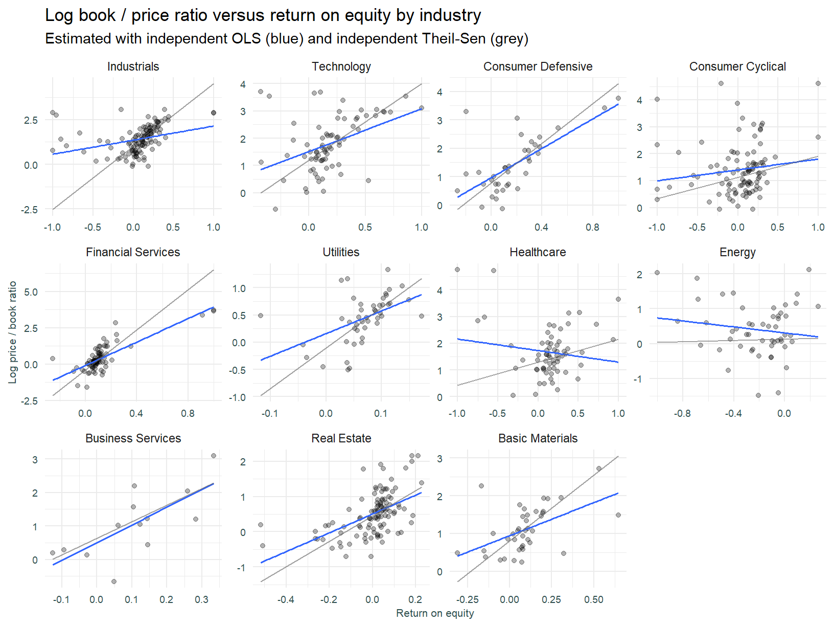
How has the line of best fit changed? Once again we might argue the robust regression fits the data better. Witness the Industrials sector. The data points distinct from the diagonal cluster skew the OLS derived slope, effectively pulling the left hand side of the line higher. The resultant slope is shallower than that derived using the Theil-Sen regression.
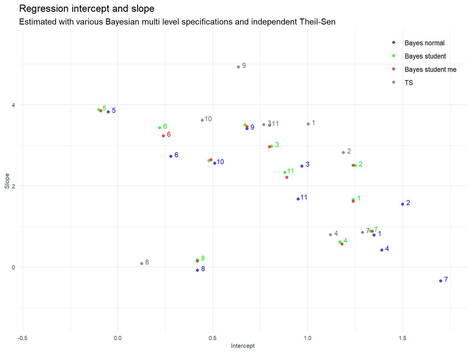
Below, we visualise the intercepts and slopes for each of the individual linear models.
The numbers assigned to sectors in this plot (and all that follow), follow the order above, i.e. 1 is Industrials and 11 is Basic Materials.
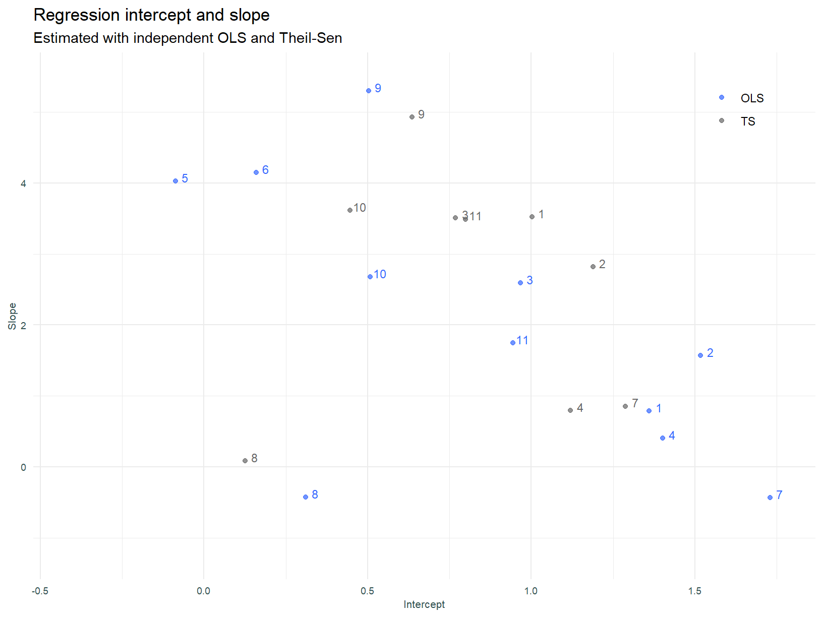
A couple of the OLS models have negative slopes, and this is counter to expectation. Consistent with the observations above, the Theil-Sen slopes are more compact or closer to each other.
Unpooled analysis - LSDV
We now add a Least Squares Dummy Variable regression. The plot below is presented with fixed scales to demonstrate the identical slopes that the LSDV structure enforces.
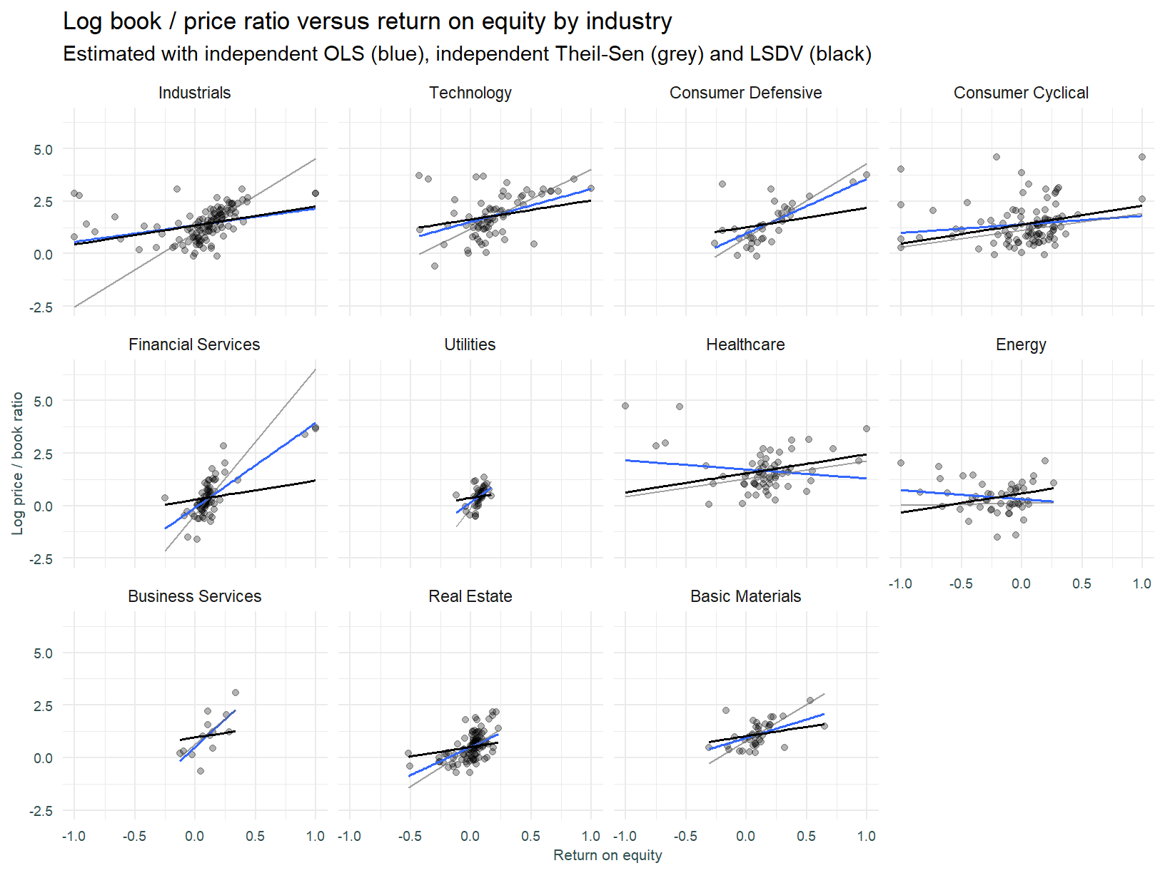
The plot is a little harder to read with the constant scale. We can see however that the LSDV forces an unnatural fit. Financial Services for example has a much smaller slope than would appear warranted. This is driven by the influence of other sectors that have a large slope. Financials are in effect an outlier among sectors and the rigidity of the model does not allow the data to influence this sectors slope.
Utilities has a comparatively compact range of returns on equity and valuations, this is consistent with a regulated industry. If a group of businesses profitability and growth is capped, variation amongst returns is constrained.
Intercepts and slopes for individual linear models by sector, and the LSDV model.
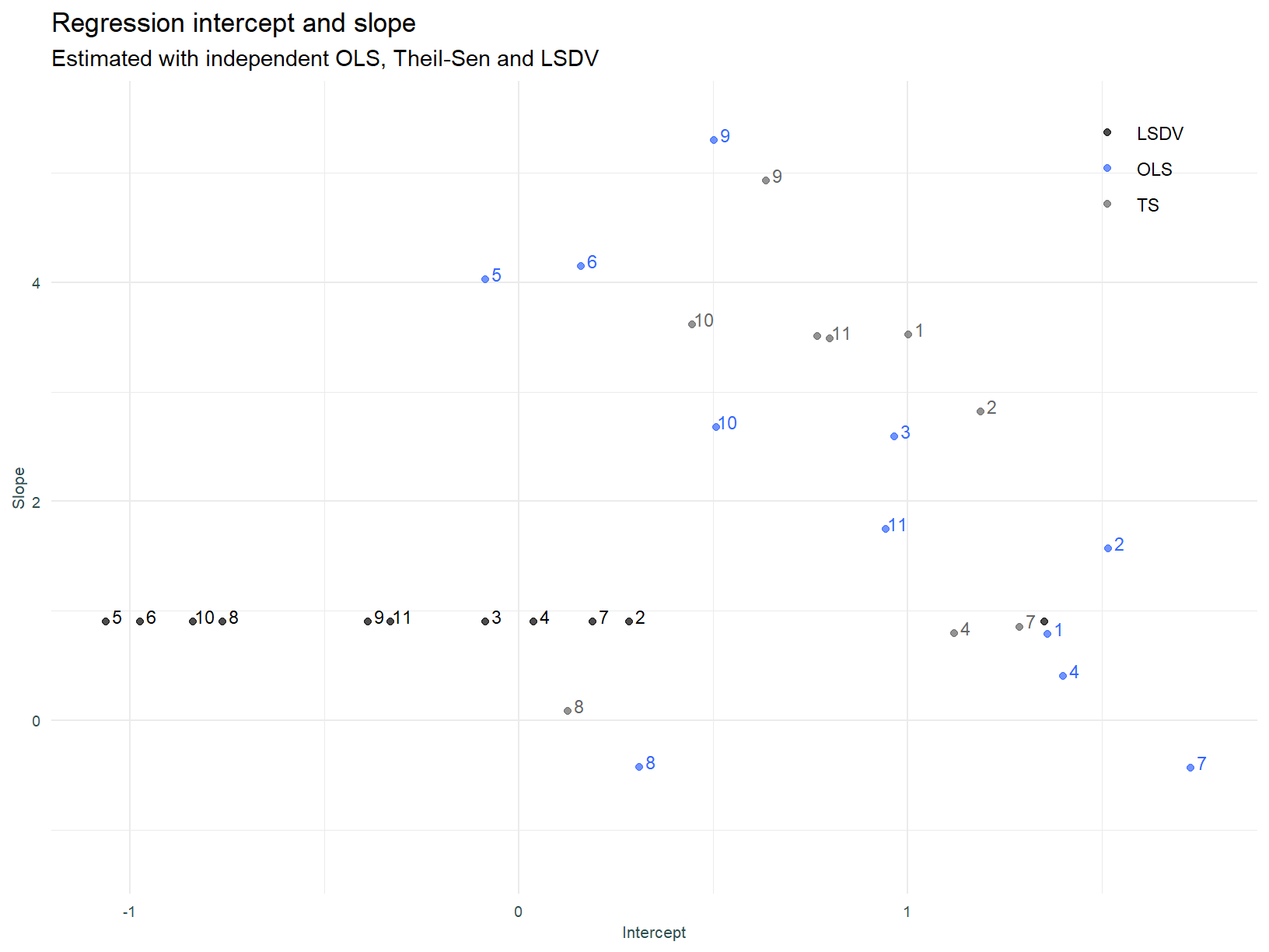
As discussed above, the LSDV model enforces a constant slope across groups and we can see this above.
Partial pooling
We now turn to multi-level models. Our expectation in fitting these types of models is that parameters will experience shrinkage to the mean as the population level data influences each groups coefficients. The references and introductory quotes inform this view.
Of interest is the extent to which the shrinkage aligns coefficients with the Theil-Sen robust model.
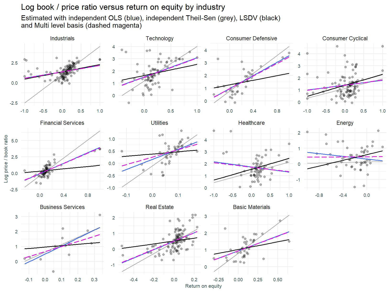
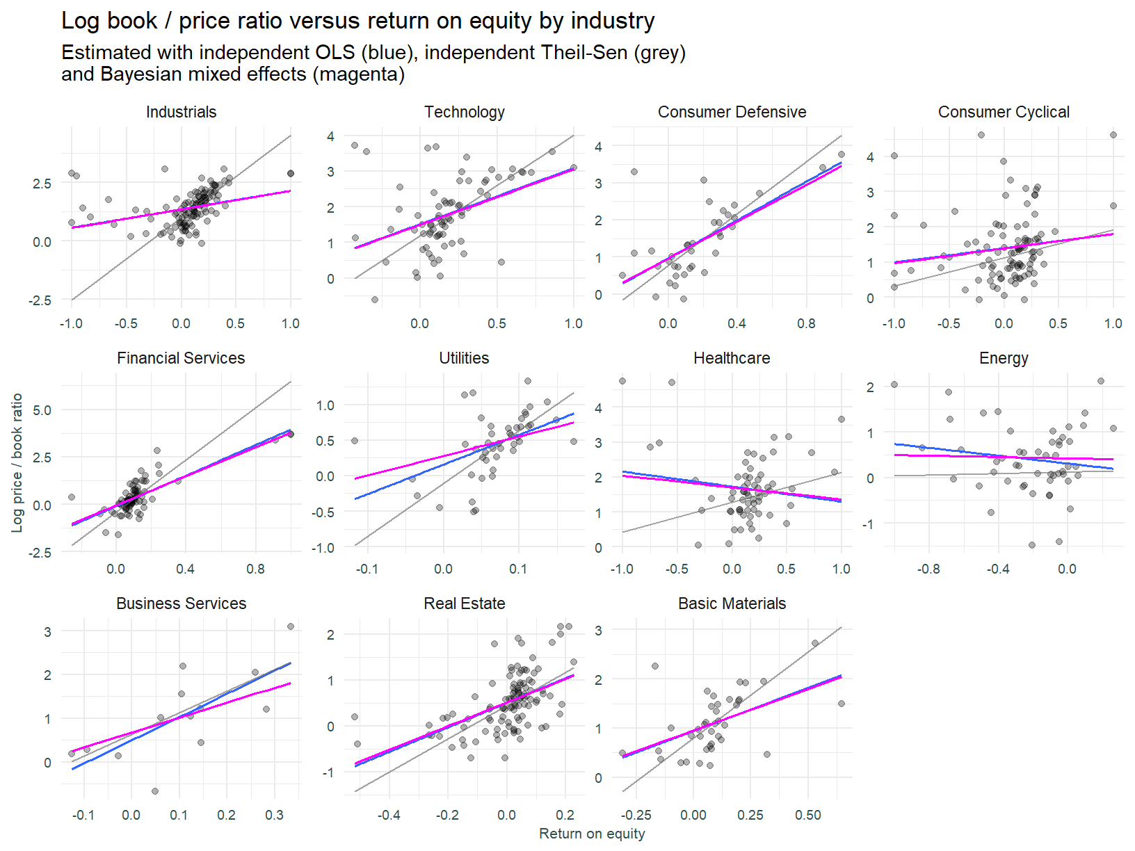
The mixed effects regression lines plotted below are estimated using the lme4 package.
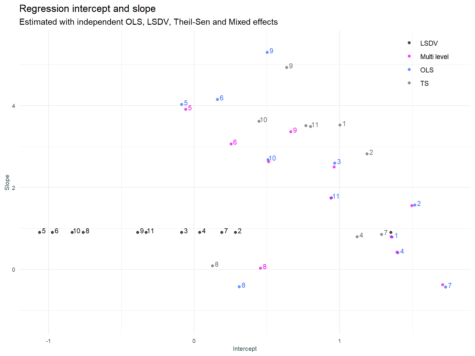
And the the coefficients.
In light of expectations, the results above are a little underwhelming. There is essentially no difference between the mixed effects and individual OLS models. Why is this so? That question should be considered in light of the drivers of parameter shrinkage in multi-level models. Shrinkage is driven by:
The size of the group, groups with more individual members will experience less shrinkage, and
The variance of the random effects (how the groups differ) versus the residual variance (how the observations within each group differ). The more groups differ, versus the extent individuals within groups differ, the less shrinkage.1
Both of these points demonstrate that these models “let the data speak”. If groups differ substantially and have a lot of members, the parameters inferred from that group remain relatively unchanged. The vice versa is true.
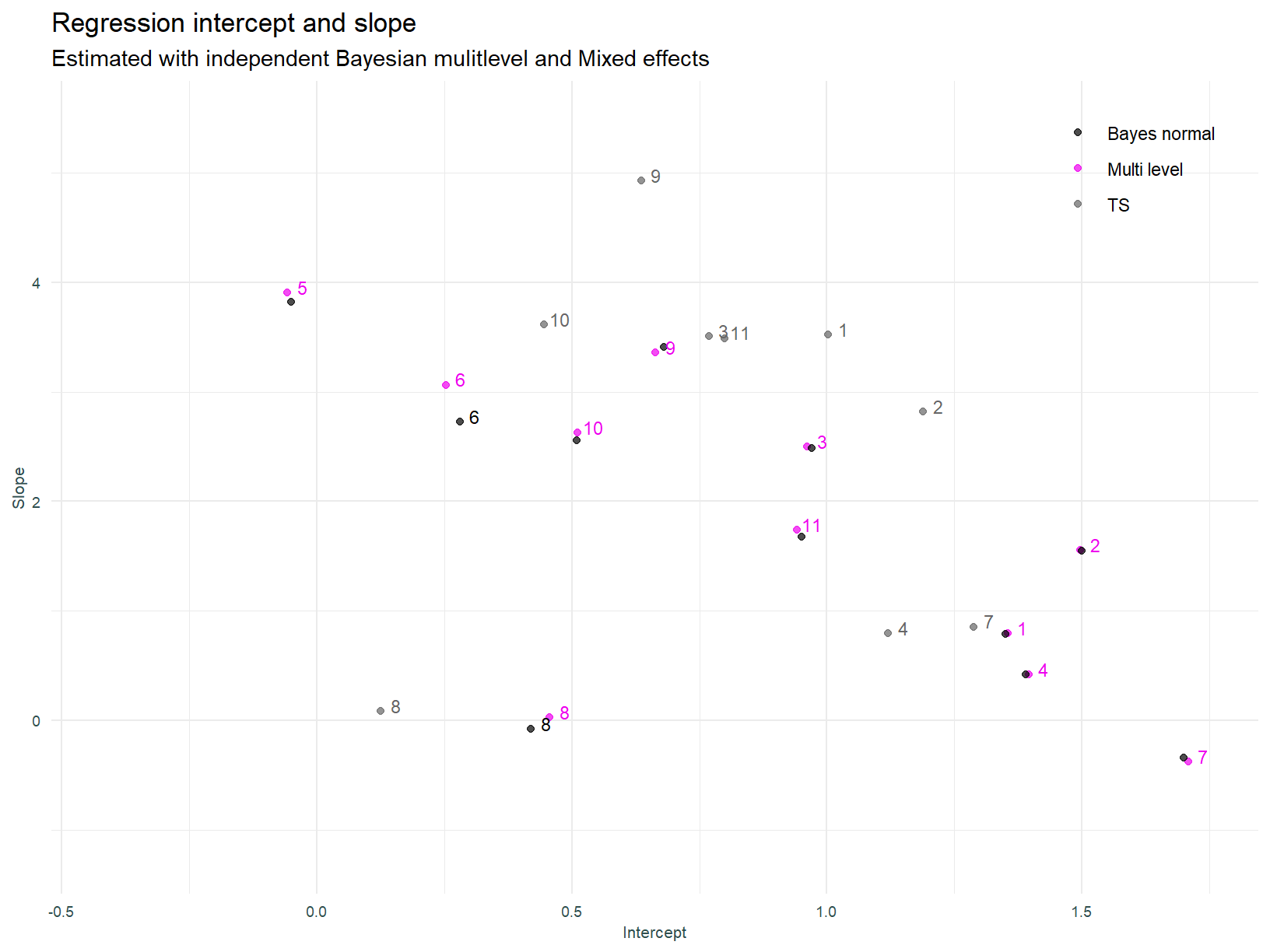
Back to the question - why so little shrinkage? This is probably due to the small number of groups (11) and the large amount of data points within each group.
Sectors that experienced the most shrinkage (the difference between the independent OLS and multi-level models) are those that have fewer data points and / or the most extreme (furthest from average) parameter estimates pre shrinkage. Sector 9 (Business Services) falls into this category.
One final point in relation to this model. As specified, the model estimates a correlation between the intercepts and slopes for each sector. Is this correlation a reasonable assumption to make in terms of model structure? Lets explore that question.
What does the intercept, or more to the point, different intercepts across sectors represent? The intercept in a regression model is the outcome when the predictor is zero. For us, the intercept is therefore the premium or discount of market value over book value, when ROE is nil.
What about the slope coefficient on ROE? Wilcox [5] at p.199 defines the slope as representing the investment horizon before the ROE reverts to its mean 2.
So, should the P/B ratio when ROE is nil systematically change with the pre mean reversion investment horizon? I’m going to say no 3.
All the same, I will continue to model using the default correlation structure, simply because it is the default behaviour for lme4 and I doubt the effect is significant.
Bayesian approach
Next, we estimate the multi-level model using a Bayesian approach. A Bayesian approach will allow for the specification of priors over both the intercept and slope coefficient, along with the correlation between those parameters. An appropriately specified prior should enforce shrinkage (if the data allows) and provides the opportunity to encode our domain knowledge. Bayesian models also allow for uncertainty quantification, however this will not be looked at with this analysis.
Let’s think about the priors. We stated above, the intercept is defined as the outcome (P/B ratio) when the predictor (ROE) is zero. So what is a reasonable expectation of the P/B ratio when ROE is zero? Ignoring the log transform initially, if an asset does not earn a return then it should not command a premium. In this case the book and market values are expected to be identical. Therefore, when ROE is zero we should expect a price to book ratio of one (the log thereof being zero). Eyeballing the second plot above largely supports this theoretical narrative.
What about the slope coefficient on ROE? As stated, we expect that the slope of the regression co-efficient is positive. All else equal, a higher ROE leads to a higher valuation.
Reflective of this, the model below therefore has a N(0, 1.5) prior for the intercept and N(1, 1.5) prior for the slope.
The Bayesian mixed effects model below is fit with the Rethinking package.
Here is the plot of the regression.
Bayesian approach - Student’s t likelihood
We now estimate the Bayesian model using tighter priors and a Student’s t likelihood. Models fitted thus far have employed a normal likelihood, the Student’s t distribution allows for fatter tails and hence for a more robust approach to dealing with outlying observations. Will this model configuration result in the un-intuitive negative slopes turning positive?
The prior over the slope in the model below is N(3, 1). The previous models prior is N(1, 1.5).
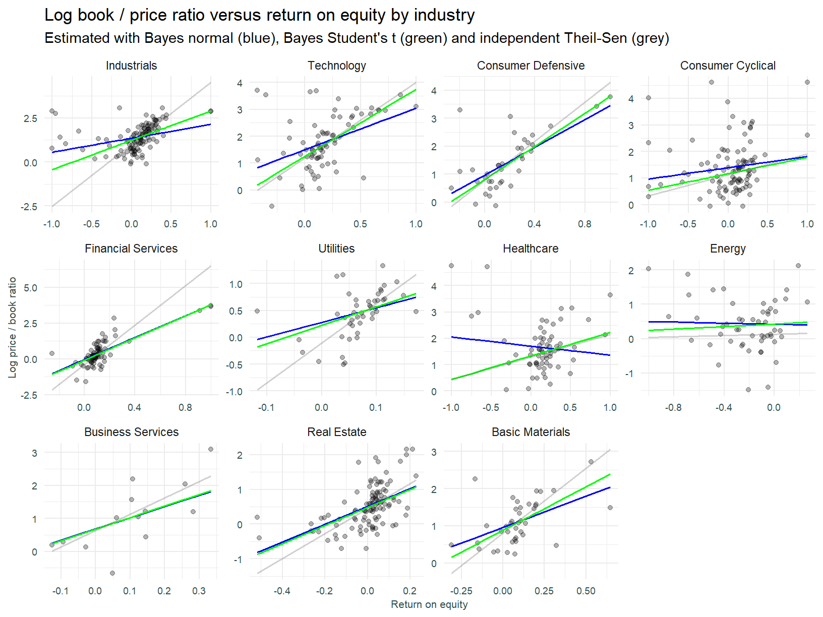
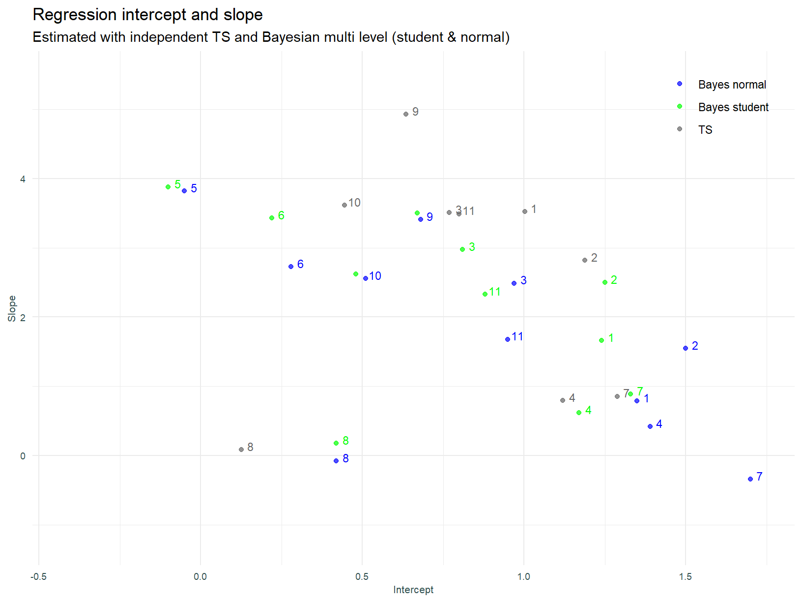
Using the Student’s t distribution does not result in drastically different slope estimates (except sector 7 - Healthcare). It is entirely possible the uncertainty around parameter estimates has been reduced (remember that is something we get with Bayesian estimation), however as stated, assessing parameter uncertainty is beyond the scope of this post.
Bayesian model with measurement error (Student’s t)
We now attempt to account for measurement error in the price to book ratio. It is well known that stock prices are more volatile than underlying business fundamentals. It is therefore reasonable to expect that any measurement error or random noise in this ratio scales with the volatility of the underlying stock price.
The model that follows is based on that per McElreath [6] p.493. This model considers the true underlying P/B ratio a function of the observed ratio and an error component that scales with trailing price volatility.
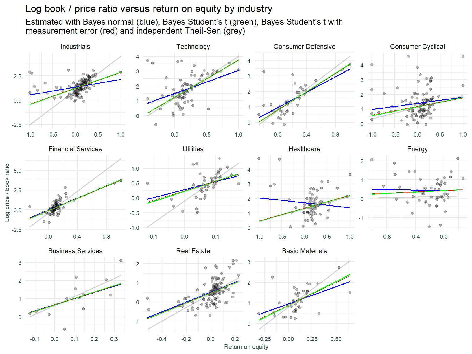
Once again, we do not see a large deviation in slope estimates across different techniques. It is difficult to pin down why this is so without performing a slew of additional analysis. I’m going to point out what I suspect is the primary issue, that being omitted variable bias. The driver of the outlying data points is a factor not modeled. The processes governing the valuation of any stock are extremely complex and noisy. We cannot hope to flexibly represent the valuation process as a model with only a single explanatory variable.
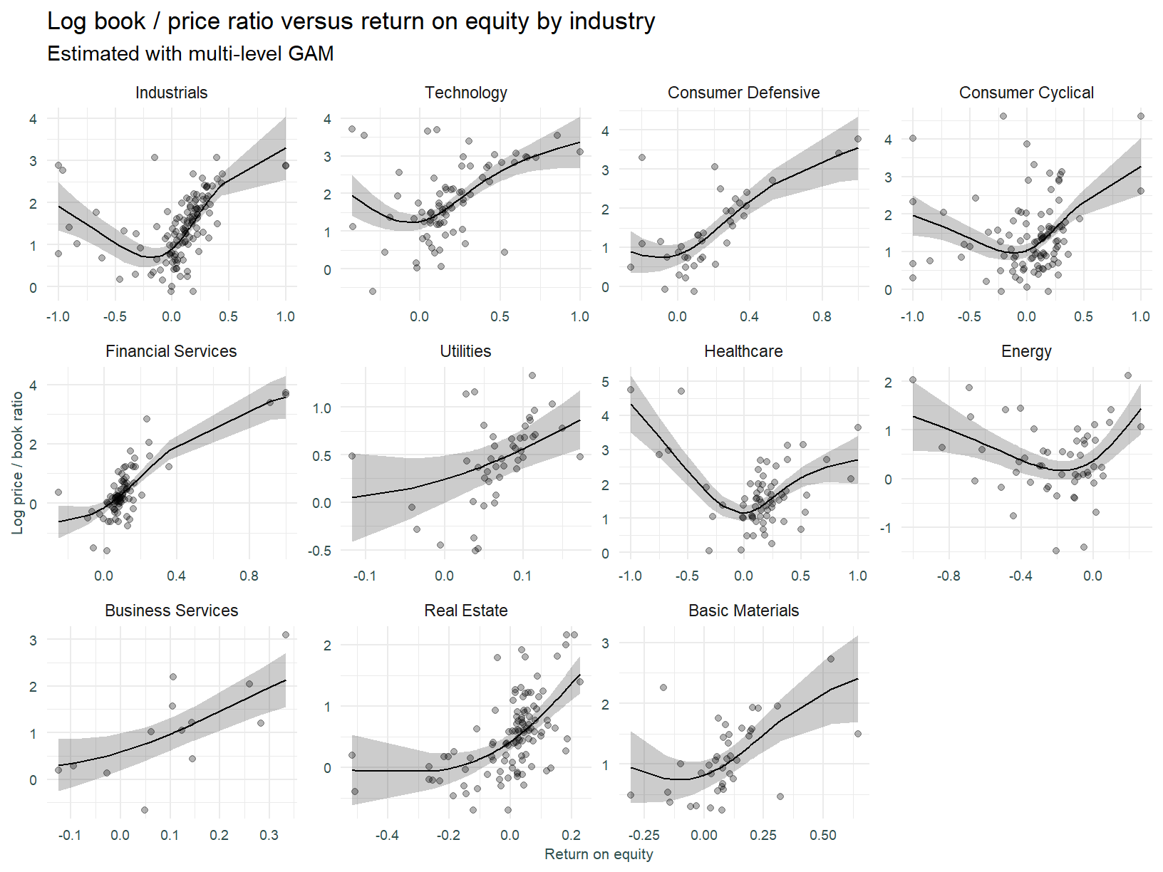
Multi-level GAM
Lastly we fit a multi-level Generalised Additive Model. The model below incorporates non-linearity, however it is constrained in that slopes (or more correctly splines) across sector must conform to a global shape. This model is of the “GS” type (global smoother with individual effects) specified in Pedersen et al. 2019 [7].
Summary
Thus far we have assessed model fit based on conformity with expectations and eyeballing of scatter plots and fitted regression lines. To summarise the various model configuration performance, lets look at each model from a predicted vs actual and predicted vs residual perspective. This may tease out further insights.
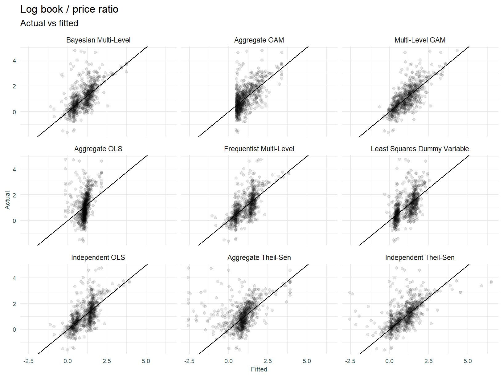
The multi-level GAM and independently fit Theil-Sen models appear to be the best fitting models.
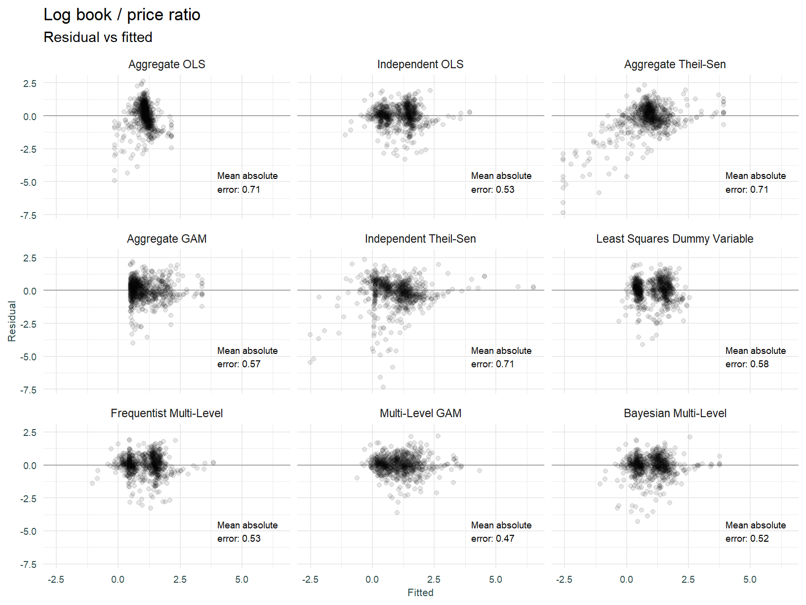
A well fitted model will have its residuals plotting an equal variance about the zero line, doing so across all values of the predicted response. This is obviously not the case for the models above, there is quite a bit of clustering of errors. We can say the multi-level GAM and Bayesian multi-level models look best.
Closing
We set out to gain an intuition over various regression modeling techniques using real data, applied to a real problem. That has been achieved with Bayesian, frequentist and robust techniques having been applied in a stock valuation setting. This post was not designed to genuinely find a useful stock valuation model, that is of course highly complex and out of scope for this short note. It is rather a means to an end, that being to understanding how different models work and getting the hands dirty with real data.
As always, a bunch of modeling considerations have not been covered:
As stated, modeling a complex phenomenon like stock valuations will be grossly under-specified with a single explanatory variable.
Bayesian models provide parameter uncertainty quantification. This has not been analysed.
The suitability of the multi-level structure has not been assessed. This could be performed with the intraclass-correlation coefficient (ICC).
Formal model comparison and model fit diagnostics has not been performed.
I’ll close with the question as to whether deviations from modeled valuation (of a more sophisticated variety, taking account of say growth and risk) correlate with future returns? Something for the next round of analysis.
References
[1] Harrison XA, Donaldson L, Correa-Cano ME, Evans J, Fisher DN, Goodwin CED, Robinson BS, Hodgson DJ, Inger R. 2018. A brief introduction to mixed effects modelling and multi-model inference in ecology. PeerJ 6:e4794 https://doi.org/10.7717/peerj.4794
[2] Paul-Christian Burkner. Advanced Bayesian Multilevel Modeling with the R Package brms. 2018
[3] Green, Brice and Thomas, Samuel, Inference and Prediction of Stock Returns using Multilevel Models (August 31, 2019). Available at SSRN: https://ssrn.com/abstract=3411358 or http://dx.doi.org/10.2139/ssrn.3411358
[4] Sommet, N. and Morselli, D., 2021. Keep Calm and Learn Multilevel Linear Modeling: A Three-Step Procedure Using SPSS, Stata, R, and Mplus. International Review of Social Psychology, 34(1), p.24. DOI: http://doi.org/10.5334/irsp.555
[5] Wilcox, J. 1999. Investing by the Numbers (Frank J. Fabozzi Series). Wiley
[6] McElreath, R. 2020. Statistical Rethinking: A Bayesian Course with Examples in R and STAN, 2nd Edition. CRC Press
[7] Pedersen EJ, Miller DL, Simpson GL, Ross N. 2019. Hierarchical generalized additive models in ecology: an introduction with mgcv. PeerJ 7:e6876 https://doi.org/10.7717/peerj.6876
[8] Various websites referenced containing background materials
This can be measured with the intraclass-correlation coefficient (ICC) / variance partition coefficient (VPC). A high ICC indicates that observations depend on cluster membership, and hence will experience less shrinkage. A low ICC / VPC can indicate that a multi-level modelling structure is not warranted. Also note the Design Effect discussed by Sommet & Morselli [4] that is designed to perform the same task.↩︎
The intuition behind this is beyond me, and the mathematics supporting the PB-ROE model are pretty hairy.↩︎
Although I can entertain the idea that P/B ratio is driven by growth in ROE across sector, and this may relate to investment horizon.↩︎