This series of posts will deal with the preparation of International Financial Reporting Standard 9 - Financial Instruments (“IFRS9”) disclosures for a bank. In particular, the reconciliation tables that are required to account for movements in loan balances and expected credit losses over a reporting period.
This is a somewhat arcane topic. Why do we want to do this?
IFRS9 is a relatively new accounting standard and the reconciliation tables disclose a flow of loan balances over time, accounting for draw downs, repayments and other cash flows. This contrasts to pre IFRS9 disclosures which for the most part disclose loan and related balances at a point in time. Preparing these type of disclosures requires complex data transformation and data modelling which can be executed in R using the dplyr package. Preparing the IFRS9 disclosures on a novel data set will provide practice in data exploration, cleaning, transformation and modelling skills using R. In addition, this will also provides an excellent opportunity to learn the same skills in Python using the pandas library.
The problem statement
We have been asked to prepare the IFRS9 disclosures for a bank (let’s call it “Bank1000”). Bank1000 will exclusively provide all debt financing to the top 1,000 US companies by market capitalisation. Therefore, when a company leaves the top 1,000 stocks by market capitalisation, it pays back its debt to Bank1000 and refinances its debt with another bank. Similarly, if a company joins the top 1,000 and has debt, it refinances that debt with Bank1000.
Bank1000 must comply with IFRS9 and related disclosures. This means it must divide its loan portfolio of 1,000 borrowers into 3 risk stages, and having chosen to use the individual as opposed to the collective expected credit loss (“ECL”) assessment method, estimate an ECL for each loan.
In addition, Bank1000 is required to prepare the disclosures mentioned above, providing a reconciliation of the opening and closing ECL and loan balance amounts. These disclosures are to be segmented by the 3 risk stages, detailing transfers between stages.
The requirements of IFRS 9 are nicely summarised by the BIS in this document, IFRS 9 and expected loss provisioning - Executive Summary (pdf). The reconciliation disclosures mentioned above have come to resemble something like the table format below, this is from EY Illustrative disclosures for IFRS9 (pdf).
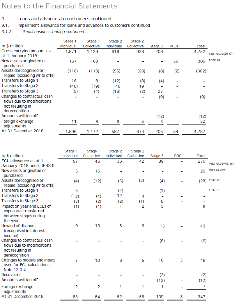
In order to perform this exercise we will need fundamental data on U.S. companies. The debt liabilities of the companies we collect data on will represent the loan gross carrying amount asset amount shown above.
The remainder of this post will deal with data acquisition and exploratory data analysis. Future posts will look at creating an expected credit loss balance and risk stage, and finally modelling the disclosures referred to above.
Financial data
It is well known that it is difficult to obtain free fundamental data on US companies. Fortunately the authors of SimFin want to change this and have granted access to data collected through automated web scraping processes. SimFin allows for a bulk download of price and fundamental data for around 2,000 U.S. companies. I have saved this bulk download to my local hard drive (this data was downloaded in October 2018).
Let’s get started exploring this data. Load the required packages,
library("tidyverse")
library("lubridate")
library("tibbletime")
library("tsibble")
library("scales")
library("DescTools")
library("ggiraphExtra")
library("cowplot")
library("kableExtra")
read the data downloaded from the SimFin website,
# Read from csv - readr
simfin <- as_tibble(read_csv(file="C:/Users/brent/Documents/R/R_import/output-comma-narrow.csv")) %>%

  # Rename attributes
  rename_all(list(~str_replace_all(., " ", "."))) %>%
  rename(Industry = Company.Industry.Classification.Code)
and view the data structure.
head(simfin)## # A tibble: 6 x 6
## Ticker SimFin.ID Industry Indicator.Name publish.date Indicator.Value
## <chr> <int> <int> <chr> <date> <dbl>
## 1 ICUI 550676 106003 Revenues 2007-10-25 44.9
## 2 ICUI 550676 106003 COGS 2007-10-25 25.5
## 3 ICUI 550676 106003 SG&A 2007-10-25 11.5
## 4 ICUI 550676 106003 R&D 2007-10-25 2.23
## 5 ICUI 550676 106003 EBIT 2007-10-25 5.65
## 6 ICUI 550676 106003 Interest expense,~ 2007-10-25 0There are just over 11 million records.
glimpse(simfin)## Observations: 11,069,838
## Variables: 6
## $ Ticker <chr> "ICUI", "ICUI", "ICUI", "ICUI", "ICUI", "ICUI"...
## $ SimFin.ID <int> 550676, 550676, 550676, 550676, 550676, 550676...
## $ Industry <int> 106003, 106003, 106003, 106003, 106003, 106003...
## $ Indicator.Name <chr> "Revenues", "COGS", "SG&A", "R&D", "EBIT", "In...
## $ publish.date <date> 2007-10-25, 2007-10-25, 2007-10-25, 2007-10-2...
## $ Indicator.Value <dbl> 44.8680, 25.5020, 11.4850, 2.2340, 5.6470, 0.0...Attributes reported on are as follows.
unique(simfin$Indicator.Name)## [1] "Revenues" "COGS"
## [3] "SG&A" "R&D"
## [5] "EBIT" "Interest expense, net"
## [7] "Abnormal Gains/Losses" "Income Taxes"
## [9] "Net Income from Discontinued Op." "Net Profit"
## [11] "Gross Margin" "Operating Margin"
## [13] "Net Profit Margin" "Common Shares Outstanding"
## [15] "Avg. Basic Shares Outstanding" "Avg. Diluted Shares Outstanding"
## [17] "Dividends" "Cash and Cash Equivalents"
## [19] "Receivables" "Current Assets"
## [21] "Net PP&E" "Intangible Assets"
## [23] "Goodwill" "Total Noncurrent Assets"
## [25] "Total Assets" "Short term debt"
## [27] "Accounts Payable" "Current Liabilities"
## [29] "Long Term Debt" "Total Noncurrent Liabilities"
## [31] "Total Liabilities" "Preferred Equity"
## [33] "Share Capital" "Treasury Stock"
## [35] "Retained Earnings" "Equity Before Minorities"
## [37] "Minorities" "Total Equity"
## [39] "Depreciation & Amortisation" "Change in Working Capital"
## [41] "Cash From Operating Activities" "Net Change in PP&E & Intangibles"
## [43] "Cash From Investing Activities" "Cash From Financing Activities"
## [45] "Net Change in Cash" "Current Ratio"
## [47] "Liabilities to Equity Ratio" "Debt to Assets Ratio"
## [49] "EBITDA" "Free Cash Flow"
## [51] "Return on Equity" "Return on Assets"
## [53] "Share Price" "Market Capitalisation"
## [55] "EV / Sales" "Book to Market"
## [57] "Operating Income / EV" "Enterprise Value"
## [59] "EV / EBITDA"There are two price related attributes, Share Price and Market Capitalisation. The remaining attributes are fundamental or accounting balances and metrics derived therefrom.
Initial checks on the data
Let’s commence exploring this data by performing some checks. The code below looks for duplicates across Ticker, Indicator.Name and publish.date.
df.dupes.1 <- simfin %>% group_by(Ticker, Indicator.Name, publish.date) %>%
  filter(n() > 1) %>% arrange(Ticker, Indicator.Name, publish.date)

head(df.dupes.1)
## # A tibble: 6 x 6
## # Groups: Ticker, Indicator.Name, publish.date [3]
## Ticker SimFin.ID Industry Indicator.Name publish.date Indicator.Value
## <chr> <int> <int> <chr> <date> <dbl>
## 1 AGN 442340 106005 Abnormal Gains/Lo~ 2014-08-05 0
## 2 AGN 61474 106005 Abnormal Gains/Lo~ 2014-08-05 0
## 3 AGN 442340 106005 Abnormal Gains/Lo~ 2014-11-05 0
## 4 AGN 61474 106005 Abnormal Gains/Lo~ 2014-11-05 0
## 5 AGN 442340 106005 Accounts Payable 2014-08-05 300
## 6 AGN 61474 106005 Accounts Payable 2014-08-05 2443.The table above indicates that there are multiple stocks with the same ticker. For example the entries under ticker ARMK (not shown above but identified after interrogating the underlying data frame) are distinguished by SimFin.ID. An internet search on this ticker shows a de-listed stock labelled “ARMK.RU”. It is likely that that our data genuinely contains multiple tickers and that these are distinguished by the SimFin.ID.
Let’s see if we can confirm this and re-run the analysis including the SimFin.ID attribute in the group by clause.
# Convert date to end of month
df.dupes.2 <- simfin %>% group_by(Ticker, SimFin.ID, Indicator.Name, publish.date) %>%
  filter(n() > 1) %>% arrange(Ticker, SimFin.ID, Indicator.Name, publish.date)

head(df.dupes.2)
## # A tibble: 0 x 6
## # Groups: Ticker, SimFin.ID, Indicator.Name, publish.date [0]
## # ... with 6 variables: Ticker <chr>, SimFin.ID <int>, Industry <int>,
## # Indicator.Name <chr>, publish.date <date>, Indicator.Value <dbl>As expected there are no duplicates across this cohort of attributes.
Next, let’s check that absent the SimFin.ID, the indicator value is different. This will verify that the SimFin.ID is in fact differentiating stocks and not creating duplicates itself.
df.dupes.3 <- simfin %>% filter(Indicator.Value != 0) %>% group_by(Ticker, Indicator.Name, publish.date, Indicator.Value) %>%
  filter(n() > 1) %>% arrange(Ticker, Indicator.Name, publish.date)

head(df.dupes.3)
## # A tibble: 6 x 6
## # Groups: Ticker, Indicator.Name, publish.date, Indicator.Value [3]
## Ticker SimFin.ID Industry Indicator.Name publish.date Indicator.Value
## <chr> <int> <int> <chr> <date> <dbl>
## 1 AGN 442340 106005 Share Price 2008-12-26 23.9
## 2 AGN 61474 106005 Share Price 2008-12-26 23.9
## 3 AGN 442340 106005 Share Price 2008-12-29 24.4
## 4 AGN 61474 106005 Share Price 2008-12-29 24.4
## 5 AGN 442340 106005 Share Price 2008-12-30 25.2
## 6 AGN 61474 106005 Share Price 2008-12-30 25.2It appears that identical data is appended to different Ticker / SimFin.ID combinations. There are 25 stocks and 128176 data points in the data frame above. This indicates that one instance of the value returned is incorrect. It is highly unlikely two different stocks have the same price and fundamental data point values. Ideally we want to exclude known incorrect values, however in this situation we do not know which record to exclude. We will proceed on the basis that the market capitalisation filtering performed at a subsequent step will exclude the incorrect data.
Let’s get an idea of the number of stocks returned. The number of distinct stocks returned on an aggregated monthly basis is plotted below.
# Convert date to end of month & count stocks by month
df.plot1 <- simfin %>% mutate(me.date = ceiling_date(publish.date, unit = "month") - 1) %>%
  select(me.date, Ticker, SimFin.ID) %>% group_by(me.date) %>%
  summarise(stock.count = n_distinct(Ticker, SimFin.ID, na.rm = TRUE))

ggplot(data = df.plot1, aes(x = me.date, y = stock.count)) +
  geom_line() +
  geom_point() +
  scale_y_continuous(labels = comma) +
  labs(title = "Monthly count of stocks returned by SimFin bulk download",
       caption = "Source: SimFin bulk data download - October 2018 (https://simfin.com/)") +
  theme_grey() +
  theme(axis.title.x = element_blank(), axis.title.y = element_blank(),
        plot.caption = element_text(size = 8, color = "grey55"))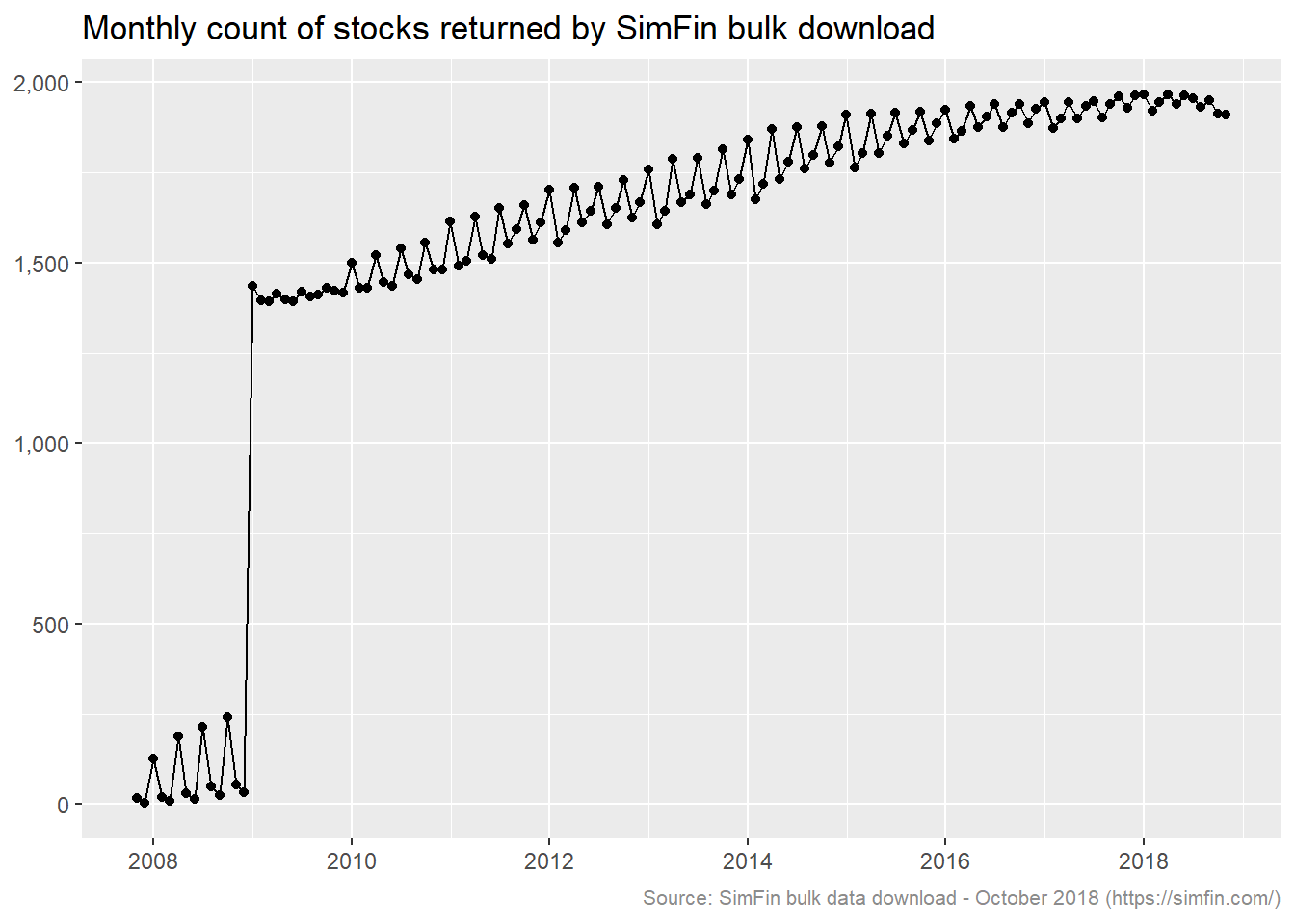
The count of stocks reaches circa 1,300 starting 2009 and gradually increases thereafter (we will ignore pre 2009 due to the count being significantly lower). The count appears to be around 100 higher on quarter end months during the years 2011 through 2015. Let’s investigate the driver of this. The code below selects all stocks with data in the months of February 2014 and March 2014, and then filters for stocks that are not in both months.
df.qtrend <- simfin %>% mutate(me.date = ceiling_date(publish.date, unit = "month") - 1) %>%
  filter(between(me.date, as.Date("2014-02-28"), as.Date("2014-03-31"))) %>%
  select(me.date, Ticker) %>% distinct() %>% mutate(value = "present") %>% spread(me.date, value) %>%
  filter(is.na(`2014-02-28`) | is.na(`2014-03-31`))
#  Dimensions and first 5 records for each category
dim(df.qtrend)
## [1] 185 3df.qtrend %>% group_by(`2014-02-28`) %>% top_n(-5, Ticker)## # A tibble: 10 x 3
## # Groups: 2014-02-28 [2]
## Ticker `2014-02-28` `2014-03-31`
## <chr> <chr> <chr>
## 1 ACPW <NA> present
## 2 ADVM <NA> present
## 3 AGIO <NA> present
## 4 ALLY <NA> present
## 5 AMCI <NA> present
## 6 BXRO present <NA>
## 7 CK00007861 present <NA>
## 8 DLTH present <NA>
## 9 FLWD present <NA>
## 10 LEN present <NA>Of the 185 cases there are 168 that have data in March 2014 and no data in February. Conversely there are 17 cases with data in February but not in March. Let’s take a case from each of the categories identified above and inspect the attributes returned for the month they are present.
simfin %>% filter(Ticker %in% c('ACPW', 'BXRO'),
           between(publish.date, as.Date("2014-02-01"), as.Date("2014-03-31"))) %>%
  select(Indicator.Name) %>% distinct(Indicator.Name)
## # A tibble: 51 x 1
## Indicator.Name
## <chr>
## 1 Common Shares Outstanding
## 2 Revenues
## 3 COGS
## 4 SG&A
## 5 R&D
## 6 EBIT
## 7 EBITDA
## 8 Interest expense, net
## 9 Abnormal Gains/Losses
## 10 Income Taxes
## # ... with 41 more rowsInspecting the underlying object reveals that there is no price or market capitalisation data available for these stocks. If there are certain stocks that have only fundamental data returned, it makes sense that more records are returned on quarter end dates when the prior quarters results are published. We will keep this lack of price data in mind as we progress.
Data periodicity
Visual inspecting of the raw SimFin data via the variable explorer reveals that the share price and market capitalisation are returned on a daily basis. Fundamental data is returned on a quarterly basis.
Let’s see if we can confirm this observation. We expect that an average of 4 data points will be returned per annum for the fundamental data attributes since these are returned quarterly. We expect circa 250 price and market capitalisation data points per annum since price is collected on weekdays.
# Convert date to year, filter for full years post 2008
df.plot2 <- simfin %>%
  mutate(ye.date = year(publish.date),
         type = case_when(Indicator.Name %in% c("Share Price", "Market Capitalisation") ~ "price",
                          Indicator.Name %in% c("Book to Market", "Total Equity", "Long Term Debt", "Short term debt", "Enterprise Value", "Total Assets", "Intangible Assets", "Revenues", "Net Profit", "Total Noncurrent Assets", "Total Noncurrent Liabilities", "Depreciation & Amortisation") ~ "fundamental",
                          TRUE ~ "not required")) %>%
  filter(type %in% c("price", "fundamental"),
         ye.date >= "2010" & ye.date <= "2017") %>%
  # Count stocks by month & ticker
  group_by(ye.date, Indicator.Name, Ticker, type) %>% summarise(value.count = n()) %>%
  group_by(ye.date, Indicator.Name, type) %>% summarise(mean.count = mean(value.count)) %>% ungroup()

df.plot2.f <- ggplot(data = df.plot2 %>% filter(type == "fundamental"),
  aes(x = Indicator.Name, y = mean.count)) +
  geom_col() + coord_flip() +
  facet_wrap(~ye.date, nrow = 2) +
  labs(title = "Fundamental data",
       caption = "Source: SimFin bulk data download - October 2018 (https://simfin.com)") +
  theme_grey() +
  theme(axis.title.x = element_blank(), axis.title.y = element_blank(),
        plot.caption = element_text(size = 9, color = "grey55"))

df.plot2.p <- ggplot(data = df.plot2 %>% filter(type == "price"),
  aes(x = Indicator.Name, y = mean.count)) +
  geom_col() + coord_flip() +
  facet_wrap(~ye.date, nrow = 2) +
  labs(title = "Price data") +
  theme_grey() +
  theme(axis.title.x = element_blank(),
        axis.title.y = element_blank(),
        axis.text.x = element_text(angle = 90))

plot_grid(df.plot2.p, df.plot2.f, align = c("h"))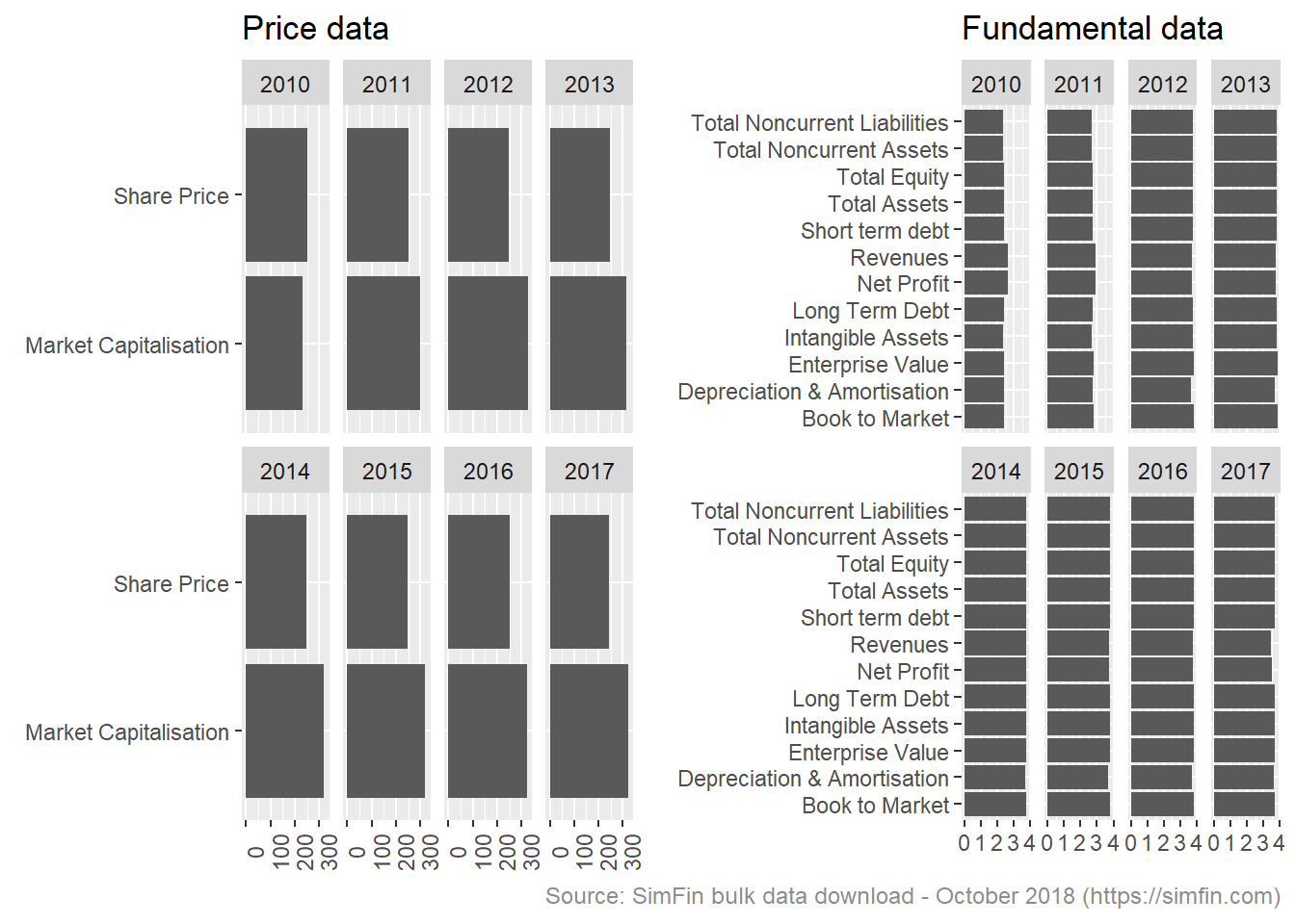
There are on average 3.8 fundamental data attribute returned per stock per year. This is in line with expectations, the count is slightly less than 4 quarterly data points reflecting the impact of de-listed stocks.
There are on average 250 share price data points returned for each stock per year. This is in line with expectation. There are on average 300 market capitalisation data points per stock per year. This exceeds the stock price data points and requires looking into.
This code block selects stocks where the count of Market capitalisation exceeds Share price.
df.check.att.1 <- simfin %>%
  filter(publish.date >= as.Date("2010-01-01") & publish.date <= as.Date("2010-12-31"),
         Indicator.Name %in% c("Share Price", "Market Capitalisation")) %>%
  # Count stocks by month & ticker
  group_by(Indicator.Name, Ticker,SimFin.ID) %>% summarise(day.count = n()) %>% ungroup() %>%
  spread(Indicator.Name, day.count) %>%
  filter(`Market Capitalisation` > 300 & `Share Price` < 260)

head(df.check.att.1, 10)
## # A tibble: 10 x 4
## Ticker SimFin.ID `Market Capitalisation` `Share Price`
## <chr> <int> <int> <int>
## 1 A 45846 310 252
## 2 AAP 184955 310 252
## 3 AAPL 111052 310 252
## 4 ABC 187024 310 252
## 5 ABCD 358762 310 252
## 6 ABT 63877 310 252
## 7 ACC 445593 310 252
## 8 ACGL 445596 310 252
## 9 ACI 646016 310 252
## 10 ACLS 670942 310 252Let’s pick one of these tickers and determine the days on which market cap is being returned and the price is not.
df.check.att.2 <- simfin %>%
  filter(publish.date >= as.Date("2010-01-01") & publish.date <= as.Date("2010-12-31"),
         Indicator.Name %in% c("Share Price", "Market Capitalisation"),
         Ticker == "AAPL") %>%
  spread(Indicator.Name, Indicator.Value) %>%
  filter(is.na(`Market Capitalisation`) | is.na(`Share Price`)) %>%
  mutate(weekday = weekdays(publish.date)) %>%
  group_by(weekday) %>% summarise(weekday.count = n())

head(df.check.att.2, 30)
## # A tibble: 5 x 2
## weekday weekday.count
## <chr> <int>
## 1 Friday 3
## 2 Monday 3
## 3 Saturday 29
## 4 Sunday 22
## 5 Thursday 1It looks like the market capitalisation is being returned on weekends and potentially public holidays. This accounts for the higher number of market cap records being returned. This is not an issue for our analysis.
Concluding on exploratory data analysis
The above analysis has identified a number of anomalies in the SimFin bulk data download. This is to be expected as it is a free data set. It should be noted that our exploratory analysis is not exhaustive, so we cannot conclude that additional anomalies do not exist. In spite of these anomalies, and given our objective of using a data set to model accounting disclosures, nothing has been identified that would prevent us from using this data for the task we have set out.
We will proceed and select the largest stocks by market capitalisation.
Filtering by market capitalisaton
We want to select the largest 1,000 companies for our imaginary loan portfolio and have decided that the indicator for determining size is market capitalisation. Let’s plot the average market capitalisation for each month for all stocks in the bulk data download. This will indicate if there are outliers or other problems in the data.
df.plot3 <- simfin %>% filter(Indicator.Name == "Market Capitalisation") %>%
  mutate(me.date = ceiling_date(publish.date, unit = "month") - 1) %>%
  select(me.date, Indicator.Value) %>%
  group_by(me.date) %>% summarise(count = n(), mkt.cap = mean(Indicator.Value)/1000)

ggplot(data = df.plot3, aes(x = me.date, y = mkt.cap)) +
  geom_line() +
  geom_point() +
  scale_y_continuous(labels = comma) +
  ylab("Market cap (millions)") +
  labs(title = "Average market capitalisation - Simfin bulk data download",
       caption = "Source: SimFin bulk data download - October 2018 (https://simfin.com/)") +
  theme_grey() +
  theme(axis.title.x = element_blank(),
        axis.title.y = element_text(color = "darkslategrey"),
        plot.caption = element_text(size = 9, color = "grey55"))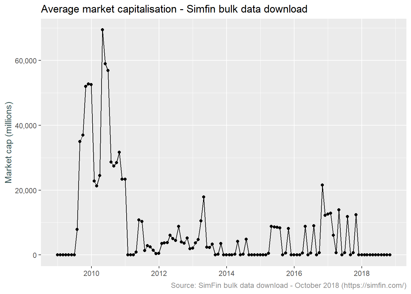
Something is obviously incorrect. For example the average market capitalisation of all stocks in February 2010 is 21 billion, this increases to 69 billion in April and by January 2011 is down to 10 thousand. The count of records for these dates is relatively consistent at 19k, 22k and 31k respectively (as mentioned earlier, market cap is provided daily and there are around 1,500 stocks). The count on the last date is higher, this will reflect the SimFin site collecting more data points over time. This last data point calls the issue out in much starker terms, the individual market capitalisation values must be drastically smaller considering the larger count and smaller value. Looking over to the forum on the SimFin site finds a number of discussion around this issue. Explanations discussed include incorrect underlying data on the SEC site, unit inconsistency and share count problems.
Given the state of the market cap data, it doesn’t appear feasible to clean this via some sort of outlier removal technique. Let’s instead infer the market value from the book to market ratio. This will entail dividing the total book equity by the book to market ratio. The code block below does just that. Note that this code pads the time series with all month end dates and fills the market cap value for each stock. This is required because the Total Equity and Book to Market values are provided quarterly, while we want to analyse data on a monthly basis.
df.plot4 <- simfin %>% filter(Indicator.Name %in% c("Book to Market", "Total Equity")) %>%

  # Remove whitespace from values, assign month end date
  mutate(Indicator.Name = str_replace_all(Indicator.Name," ",""),
         me.date = ceiling_date(publish.date, unit = "month") - 1) %>%

  # Transform attributes required for & calculate inferred market cap
  spread(Indicator.Name, Indicator.Value) %>%
  mutate(mkt.cap = TotalEquity / BooktoMarket) %>% filter(is.finite(mkt.cap)) %>%
  select(Ticker, me.date, mkt.cap) %>%

  # Pad time series for all month end dates
  complete(me.date = seq(as.Date("2008-01-01"), as.Date("2019-01-01"), by = "month") - 1, Ticker) %>%

  # Fill market cap values
  group_by(Ticker) %>% fill(mkt.cap) %>% ungroup() %>%

  # Average market cap
  group_by(me.date) %>% summarise(count = n(), mkt.cap = mean(mkt.cap, na.rm = TRUE))

# Visualise
ggplot(data = df.plot4, aes(x = me.date, y = mkt.cap)) +
  geom_line() +
  geom_point() +
  scale_y_continuous(labels = comma) +
  ylab("Market cap (millions)") +
  labs(title = "Average market capitalisation - SimFin bulk data download",
       subtitle = "Market capitalisation inferred via book to market ratio and total equity",
       caption = "Source: SimFin bulk data download - October 2018 (https://simfin.com/)") +
  theme_grey() +
  theme(axis.title.x = element_blank(),
        axis.title.y = element_text(color = "darkslategrey"),
        plot.caption = element_text(size = 9, color = "grey55"))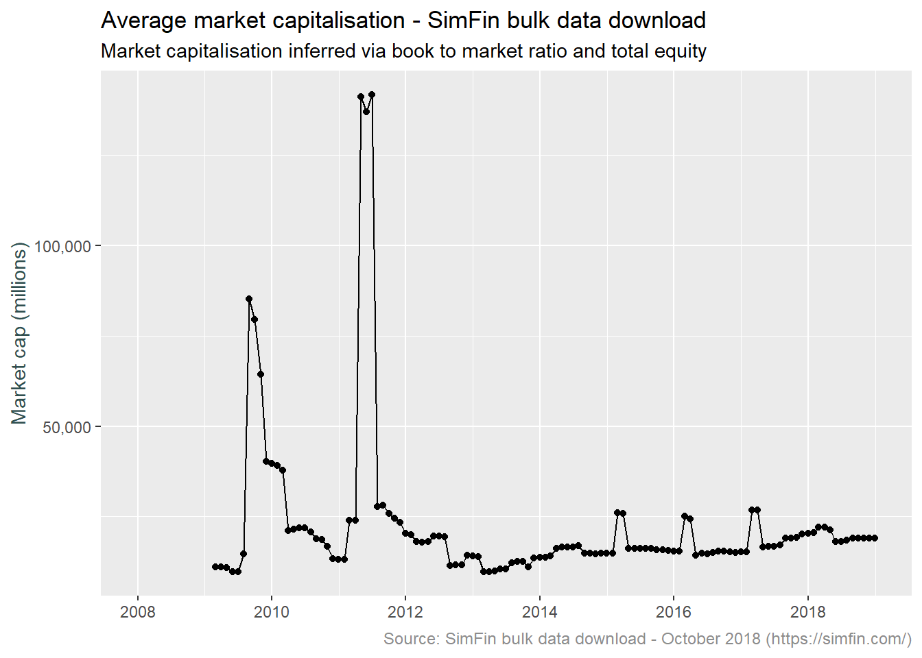
We still have some significant outliers. What is going on here? Let’s have a look at February 2017 and June 2011, the largest and most recent of the outliers shown above.
simfin %>% filter(Indicator.Name %in% c("Book to Market", "Total Equity")) %>%
  mutate(Indicator.Name = str_replace_all(Indicator.Name," ",""),
         me.date = ceiling_date(publish.date, unit = "month") - 1) %>%
  spread(Indicator.Name, Indicator.Value) %>%
  mutate(mkt.cap = TotalEquity / BooktoMarket) %>% filter(is.finite(mkt.cap)) %>%
  select(Ticker, me.date, TotalEquity, BooktoMarket, mkt.cap) %>%
  filter(me.date == "2017-02-28" | me.date == "2011-06-30") %>%
  group_by(me.date) %>% top_n(10, mkt.cap) %>% arrange(me.date, desc(mkt.cap)) %>%
  head(20)
## # A tibble: 20 x 5
## # Groups: me.date [2]
## Ticker me.date TotalEquity BooktoMarket mkt.cap
## <chr> <date> <dbl> <dbl> <dbl>
## 1 NAV 2011-06-30 -764 -0.0002 3820000
## 2 WMT 2011-06-30 68415 0.442 154680.
## 3 ORCL 2011-06-30 40245 0.271 148451.
## 4 MON 2011-06-30 12056 0.352 34260.
## 5 ACN 2011-06-30 4176. 0.124 33763.
## 6 HPQ 2011-06-30 41795 1.43 29287.
## 7 COST 2011-06-30 12541 0.453 27697.
## 8 ADBE 2011-06-30 5389. 0.350 15385.
## 9 INTU 2011-06-30 2821 0.188 14997.
## 10 A 2011-06-30 3961 0.353 11208.
## 11 HIG 2017-02-28 16903 0.001 16903000
## 12 AAPL 2017-02-28 132390 0.201 657349.
## 13 GOOG 2017-02-28 139036 0.251 554149.
## 14 BRKA 2017-02-28 296280 0.704 420733.
## 15 AMZN 2017-02-28 19285 0.0489 394376.
## 16 FB 2017-02-28 59194 0.156 378720.
## 17 XOM 2017-02-28 173830 0.549 316515.
## 18 JPM 2017-02-28 254190 0.819 310291.
## 19 GE 2017-02-28 80515 0.321 250669.
## 20 T 2017-02-28 124110 0.507 244938.It appears spurious values of the book to market ratio are driving the large values of market cap, refer to tickers NAV and HIG for June 2011 and February 2017 respectively. Let’s try again, winsorizing the Book to Market ratio over the range 0.1 to 3. This to say that whenever we see a company with a market cap greater the 10 times its book value or less than a third of its book value, we expect the underlying book to market ratio is spurious, and limit the value thereof.
df.plot5 <- simfin %>% filter(Indicator.Name %in% c("Book to Market", "Total Equity")) %>%

  # Remove whitespace from values, assign month end date
  mutate(Indicator.Name = str_replace_all(Indicator.Name," ",""),
         me.date = ceiling_date(publish.date, unit = "month") - 1) %>%

  # Transform attributes required for & calculate inferred market cap
  # Winsorize book to market ratio
  spread(Indicator.Name, Indicator.Value) %>%

  # Absolute values for correct application of min and max value
  mutate(mkt.cap = abs(TotalEquity) / Winsorize(abs(BooktoMarket), minval = 0.1, maxval = 3)) %>%
  filter(is.finite(mkt.cap)) %>% select(Ticker, me.date, mkt.cap) %>%

  # Pad time series for all month end dates
  complete(me.date = seq(as.Date("2008-01-01"), as.Date("2019-01-01"), by = "month") - 1, Ticker) %>%

  # Fill market cap values
  group_by(Ticker) %>% fill(mkt.cap) %>% ungroup() %>%

  # Average market cap
  group_by(me.date) %>% summarise(count = n(), mkt.cap = mean(mkt.cap, na.rm = TRUE))

# Visualise
ggplot(data = df.plot5, aes(x = me.date, y = mkt.cap)) +
  geom_line() +
  geom_point() +
  scale_y_continuous(labels = comma) +
  ylab("Market cap (millions)") +
  labs(title = "Average market capitalisation - SimFin bulk data download",
       subtitle = "Market capitalisation inferred via winsorised book to market ratio and total equity",
       caption = "Source: SimFin bulk data download - October 2018 (https://simfin.com/)") +
  theme_grey() +
  theme(axis.title.x = element_blank(),
        axis.title.y = element_text(color = "darkslategrey"),
        plot.caption = element_text(size = 9, color = "grey55"))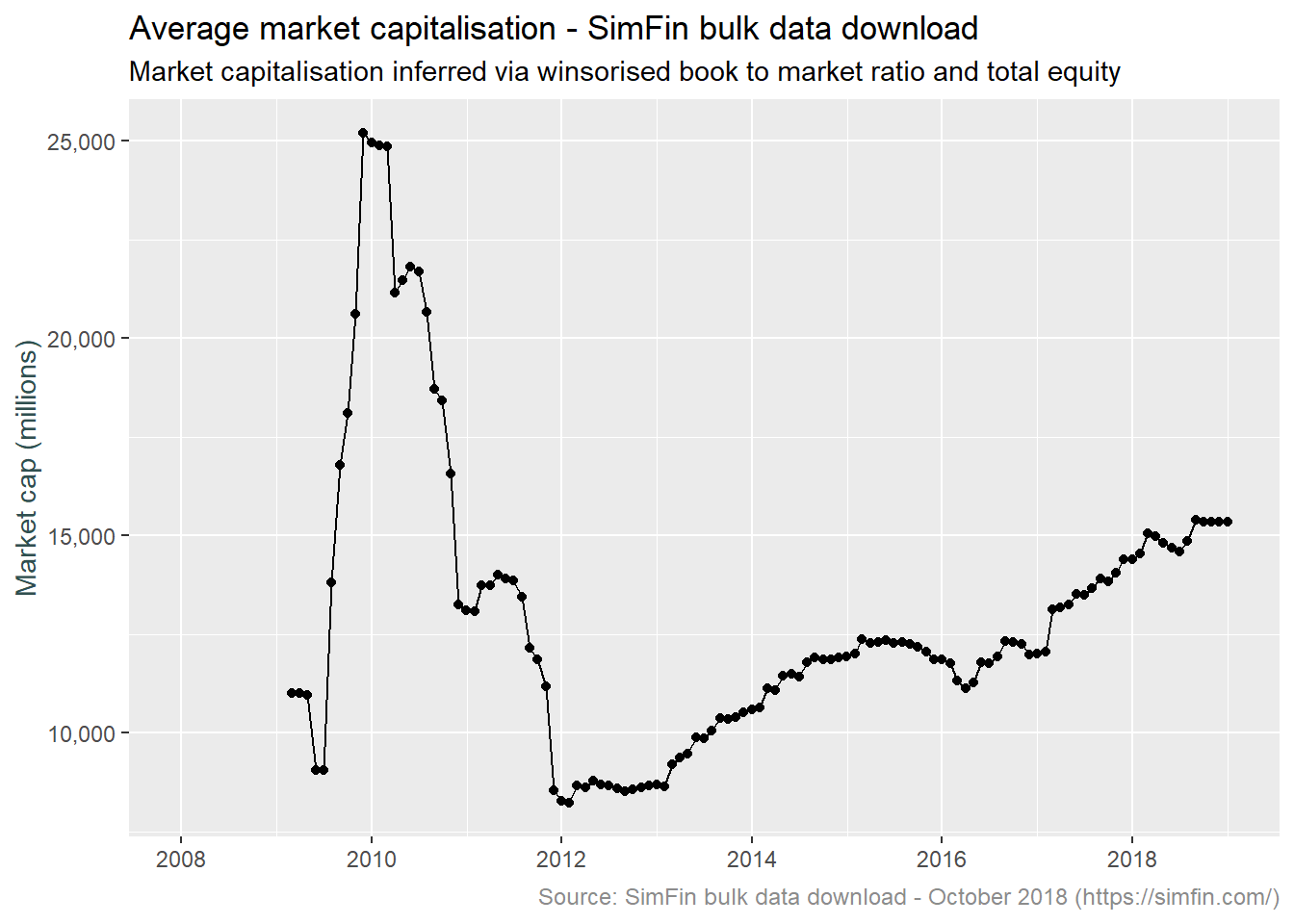
The data post January 2012 looks reasonable with the shape of the market capitalisation plot broadly following the shape of the US market proxied by the S&P 500 index. What about pre 2012? The average balances are drastically higher. Let’s compare the top 10 and bottom 10 stocks by market capitalisation for both February 2010 and February 2012. This may provide an idea as to what is driving the values returned.
# Market cap construction
mkt.cap <- simfin %>% filter(Indicator.Name %in% c("Book to Market", "Total Equity")) %>%
  mutate(Indicator.Name = str_replace_all(Indicator.Name," ",""),
         me.date = ceiling_date(publish.date, unit = "month") - 1) %>%
  spread(Indicator.Name, Indicator.Value) %>%
  mutate(mkt.cap = abs(TotalEquity) / Winsorize(abs(BooktoMarket), minval = 0.1, maxval = 3)) %>%
  filter(is.finite(mkt.cap)) %>%
  complete(me.date = seq(as.Date("2008-01-01"), as.Date("2019-01-01"), by = "month") - 1, Ticker)   %>% group_by(Ticker) %>% fill(mkt.cap) %>% ungroup() %>%
  select(Ticker, me.date, TotalEquity, BooktoMarket, mkt.cap)

#Top 10 by month
mkt.cap %>% filter(me.date == "2010-02-28" | me.date == "2012-02-29") %>%
  group_by(me.date) %>% top_n(10, mkt.cap) %>% arrange(me.date, desc(mkt.cap)) %>%
  head(20)
## # A tibble: 20 x 5
## # Groups: me.date [2]
## Ticker me.date TotalEquity BooktoMarket mkt.cap
## <chr> <date> <dbl> <dbl> <dbl>
## 1 BRKA 2010-02-28 NA NA 1357850
## 2 XOM 2010-02-28 115392 0.488 236653.
## 3 MSFT 2010-02-28 NA NA 205204.
## 4 WMT 2010-02-28 NA NA 166692.
## 5 AAPL 2010-02-28 NA NA 163175.
## 6 PG 2010-02-28 NA NA 135323.
## 7 BAC 2010-02-28 231444 1.74 133297.
## 8 IBM 2010-02-28 22755 0.172 131913.
## 9 JPM 2010-02-28 165365 1.27 130713.
## 10 GE 2010-02-28 125136 0.966 129554.
## 11 AAPL 2012-02-29 NA NA 369074.
## 12 XOM 2012-02-29 160744 0.480 334674.
## 13 MSFT 2012-02-29 NA NA 206177.
## 14 BRKA 2012-02-29 180269 0.908 198447.
## 15 IBM 2012-02-29 20235 0.107 189466.
## 16 CVX 2012-02-29 122181 0.726 168409.
## 17 WMT 2012-02-29 NA NA 167087.
## 18 GE 2012-02-29 118134 0.721 163893.
## 19 JNJ 2012-02-29 61366 0.420 146075.
## 20 PG 2012-02-29 NA NA 142450.# Bottom 10 by month
mkt.cap %>% filter(me.date == "2010-02-28" | me.date == "2012-02-29") %>%
group_by(me.date) %>% top_n(-10, mkt.cap) %>% arrange(me.date, desc(mkt.cap)) %>%
head(20)## # A tibble: 20 x 5
## # Groups: me.date [2]
## Ticker me.date TotalEquity BooktoMarket mkt.cap
## <chr> <date> <dbl> <dbl> <dbl>
## 1 LLL 2010-02-28 6660 913079. 2220
## 2 PTEN 2010-02-28 2082. 0.942 2209.
## 3 BIIB 2010-02-28 6262. 421. 2087.
## 4 NFLX 2010-02-28 199. 0.057 1991.
## 5 SLM 2010-02-28 5279. 3.07 1760.
## 6 SPXC 2010-02-28 1882. 1.18 1592.
## 7 TGNA 2010-02-28 1826. 1.21 1514.
## 8 ICUI 2010-02-28 265. 0.535 496.
## 9 PZZA 2010-02-28 185. 0.607 305.
## 10 CLX 2010-02-28 27 0.0041 270
## 11 TBTC 2012-02-29 NA NA 1.18
## 12 IMMY 2012-02-29 -1.70 -1.47 1.16
## 13 QEBR 2012-02-29 NA NA 1.12
## 14 UOLI 2012-02-29 NA NA 1.01
## 15 CYCA 2012-02-29 NA NA 0.650
## 16 FRZT 2012-02-29 NA NA 0.542
## 17 ZDPY 2012-02-29 NA NA 0.437
## 18 ADTM 2012-02-29 NA NA 0.232
## 19 CMRO 2012-02-29 NA NA 0.140
## 20 RAVE 2012-02-29 0.00631 0.0001 0.0631It should be noted that in the tables above, the NA’s are due to the fill function being applied only to the mkt.cap column as opposed to both the TotalEquity and BooktoMarket columns. In terms of the results, the market cap of the top 10 stocks appears to be consistent over the two dates. BRKA is an outlier whereby the Book to Market ratio returned at 2009-11-06 is 0.0251, this has been winsorised to 0.1 and applied to a book equity value of 135.7 billion. This results in an inferred market cap of 1.36 trillion. The bottom 10 stocks are a different story however, the 2010 values average around 1.5 billion while the 2012 values are closer to 1 million. I suspect this is due to unit inconsistency.
We are interested only in the top 1,000 stocks. The analysis above indicates the highest market cap values are relatively correct (relative in the sense that the BRKA outlier referred to above does not invalidate our goal of selecting the top 1,000 stocks). We are not sure if the suspected unit inconsistency for low capitalisation stocks extends to the 1,000th value however. If we can plot a time series of say the 5th and 1,000th values of market capitalisation, and these do not significantly diverge, we can conclude the top 1,000 is relatively correct. This is good enough for our purposes.
# Market cap construction
mkt.cap %>% filter(!is.na(mkt.cap)) %>% nest(-me.date) %>%
  mutate(fifth = map(data, ~nth(.$mkt.cap, -5L, order_by = .$mkt.cap)),
         thousandth = map(data, ~nth(.$mkt.cap, -1000L, order_by = .$mkt.cap))) %>%
  filter(me.date > "2012-12-31") %>% select(-data) %>%
  gather(key, value, fifth, thousandth) %>% mutate(value = as.numeric(value)) %>%
  ggplot(aes(x = me.date, y = value, colour = key)) +
  facet_grid(key ~ ., scales = 'free') +
  scale_y_continuous(labels = comma) +
  ylab("Market cap (millions)") +
  labs(title = "Market capitalisation for the fifth and thousandth largest stock",
       subtitle = "Market capitalisation inferred via winsorised book to market ratio and total equity",
       caption = "Source: SimFin bulk data download - October 2018 (https://simfin.com/)") +
  geom_line() +
  theme_grey() +
  theme(legend.position = "none") +
  theme(axis.title.x = element_blank(),
        axis.title.y = element_text(color = "darkslategrey"),
        plot.caption = element_text(size = 9, color = "grey55"))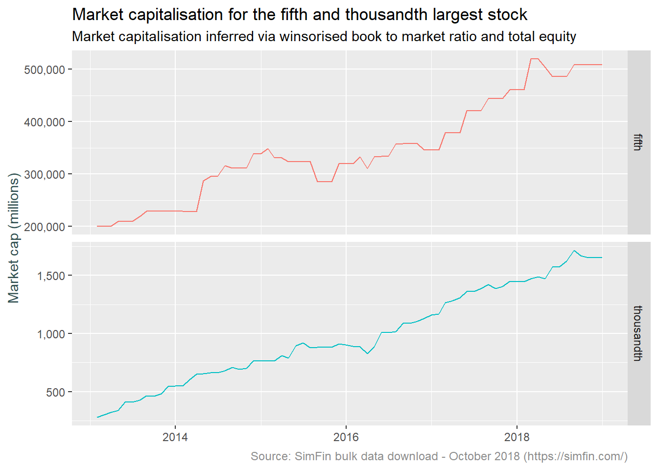
This we can work with. The drift higher in the fifth and thousandth largest stocks mirrors the overall market over the post 2012 period.
The code block below creates a data frame containing market capitalisation cut-off points to be used in selecting stocks.
# Stock market cap filter construction
mkt.cap.filter <- mkt.cap %>% filter(!is.na(mkt.cap)) %>% nest(-me.date) %>%
  mutate(thousandth     = map(data, ~nth(.$mkt.cap, -1000L, order_by = .$mkt.cap)),
         eighthundredth = map(data, ~nth(.$mkt.cap, -800L, order_by = .$mkt.cap)),
         sixhundredth   = map(data, ~nth(.$mkt.cap, -600L, order_by = .$mkt.cap)),
         fourhundredth  = map(data, ~nth(.$mkt.cap, -400L, order_by = .$mkt.cap)),
         twohundredth   = map(data, ~nth(.$mkt.cap, -200L, order_by = .$mkt.cap))) %>%
  filter(me.date > "2012-12-31") %>% select(-data) %>% unnest()
Conclusion and next steps
The purpose of this post is to source and analysis fundamental data for U.S. companies with a view to using this data to model IFRS9 disclosures. To this end we have downloaded the SimFin bulk data set and explored same noting several data anomalies.
We have concluded that the raw market capitalisation data is not suitable for determining the top 1,000 stocks, and instead inferred market capitalisation from the book to market ratio and total equity. This data has then been used to create a monthly time series of market cap cut-off points for various quantiles.
The next post will look at creating an expected credit loss balance and risk stage. This will allow us to conclude with the ultimate aim of modelling the IFRS9 disclosures outlined above.