This post documents an exploratory data analysis that assesses the relationship between the slope of the yield curve and the S&P 500 index. We will discretise the yield curve into equal frequency bins based on its level and change and draw a histogram of the subsequent S&P 500 returns associated with each bin. We will also prepare a plot visualising periods when future S&P 500 returns are within specific parameters. The source data for this post is the script documented here.
Background
The yield curve, calculated as the spread between the Federal funds rate and the 10-year Treasury note rate, is theorized to be a powerful indicator of the business cycle (wikipedia reference). What interests us is not the economic cycle, but whether the yield curve is an early indicator for the stock market. Does a certain level, change (or combination of these) of the yield curve provide information about future stock market returns? For example, if the yield curve is in the bottom third of its historical range and rises, are the following stock market returns different from other periods?
The logic for using a discretisation approach as opposed to fitting and interpreting regression coefficients is motivated by the expectation of nonlinearities in the relationship between the yield curve and the stock market. If the inversion of the yield curve is seen as a signal for lower future economic activity, as theorized above, then the state of the yield curve is not expected to be relevant at other times. If we can determine these time periods, we might be able to add suitable interaction conditions to deal with nonlinearities when we return to regression models.
Data preparation
We start by loading the required packages and the previously prepared data.
library("tidyverse")
library("cowplot")
library("caret")
library("scales")

econ_fin_data <- readRDS("econ_fin_data.Rda")
sp_shade      <- readRDS("sp_shade.Rda")
Next, we calculate the yield curve by subtracting the Federal funds rate from the 10-year Treasury rate. We then categorize the yield curve into bins that represent specific levels and change values. The following code block breaks down the time series of the yield curve into 6 bins. The yield curve level is divided into terciles or three bins with the same number of months. The change in level is categorised as either a rise or a fall (positive or negative 6-month change). The combination of these two is then lagged by 6 months and 12 months, resulting in a total of 18 bins. Three bins will be triggered at any point in time.
# create the yield curve time series (designated "ff_10")
x2 <- econ_fin_data %>% mutate(ff_10 = GS10 - FEDFUNDS) %>%

  # select data required, including indicator under analysis
  select(date, close, fwd_rtn_m, ff_10) %>%

  # lagged values of indicator under analysis
  mutate(x1.lag6  = lag(ff_10, 6),
         x1.lag12 = lag(ff_10, 12),

         # tercile level factor
         x1.qntlx = ntile(ff_10, 3),
         x1.qntl = case_when(x1.qntlx == 1 ~ "_low",
                             x1.qntlx == 2 ~ "_mid",
                             x1.qntlx == 3 ~ "_high"),

         # change in level indicator
         x1.rtn6  = ff_10 - x1.lag6,
         x1.rtn12 = ff_10 - x1.lag12,

         # binary change in level factor
         x1.delta = if_else(ff_10 > lag(ff_10, n = 6),
                            "incr",
                            "decr")) %>%

  # factor combining tercile level and binary change in level factors
  unite(x1_lag00, c(x1.qntl, x1.delta),sep = "_", remove = FALSE) %>%

  # lagged combined factor and filter out NA's
  mutate(x1_lag06 = lag(x1_lag00, 6),
         x1_lag12 = lag(x1_lag00, 12)) %>%
  filter(!is.na(x1.lag12))
This code block retrieves the current status of each of the three levels/change bins.
# current values of factor values for plot text
x2.1 <- slice(x2, n()) %>% select(x1_lag00, x1_lag06, x1_lag12) %>% t() %>%
  data.frame() %>% rownames_to_column() %>%
  unite(Indicator, c(rowname, .), sep = "", remove = TRUE) %>%
  mutate(Indicator =  gsub("x1_", "", Indicator))

# view current values
str(x2.1)
## 'data.frame': 3 obs. of 1 variable:
## $ Indicator: chr "lag00_low_decr" "lag06_mid_decr" "lag12_mid_incr"Three strings are returned, the current and two lagged values. Note the format of these strings, this will be used later in the histogram. The first five characters indicate whether the bin series is current or delayed, the middle three characters indicate the level tercile, and finally we have the change in level indicator.
Remember that we would like to draw a histogram of the subsequent S&P 500 returns. To enable segmentation for the histogram, we need to create dummy variables for each of the 18 bins. This is where the caret package comes in handy.
# dummy variables for each (current & lagged) combined level / change factor
x3 <- predict(dummyVars(" ~ x1_lag00", data = x2), newdata = x2)
x4 <- predict(dummyVars(" ~ x1_lag06", data = x2), newdata = x2)
x5 <- predict(dummyVars(" ~ x1_lag12", data = x2), newdata = x2)

# combine dummy variable sets (current and lagged) to single data frame
x6 <- as.tibble(cbind(x3, x4, x5)) %>% select(-contains("NA")) %>%
  rownames_to_column(var = 'rowIndex') %>%

  # transform combined dummy variable data from wide to long format
  gather(key = 'Indicator', value = 'Value', -rowIndex) %>%

  # convert dummy variable to factor
  mutate(Value_fact = ifelse(Value == 1, "In", "Out"))

# assign rownames to columns in order to join return data to dummy variable data
x7 <- x2 %>% select(date, fwd_rtn_m) %>% rownames_to_column(var = 'rowIndex')

# data for histogram plot - join return data to dummy variable data
x8 <- full_join(x6, x7, by  = 'rowIndex') %>%
  # rename indicator
  mutate(Indicator = str_replace(Indicator, "x1_", "ff_10 : "))
We now have a table with 18 records for each date, six for each of the current and two delayed level/change bins as previously defined. Three of them are labelled “In”, one of the six of each of the current and two lagged values, these represent the status of the yield curve at that date. All other records are labelled “Out”. These are our dummy variables. The table also contains the monthly return of the S&P 500 for the month following the designation. The histogram is derived from this table.
library("knitr")
library("kableExtra")
x8 %>% filter(date == "2019-03-01") %>% select(date, fwd_rtn_m, Indicator, Value_fact) %>%
  kable(align = "c") %>%  kable_styling(bootstrap_options = c("striped", "responsive")) %>%
  column_spec(1, width = "5cm") %>% column_spec(2, width = "4cm") %>%
column_spec(3, width = "8cm") %>% column_spec(4, width = "5cm")| date | fwd_rtn_m | Indicator | Value_fact |
|---|---|---|---|
| 2019-03-01 | 0.0246135 | ff_10 : lag00_high_decr | Out |
| 2019-03-01 | 0.0246135 | ff_10 : lag00_high_incr | Out |
| 2019-03-01 | 0.0246135 | ff_10 : lag00_low_decr | In |
| 2019-03-01 | 0.0246135 | ff_10 : lag00_low_incr | Out |
| 2019-03-01 | 0.0246135 | ff_10 : lag00_mid_decr | Out |
| 2019-03-01 | 0.0246135 | ff_10 : lag00_mid_incr | Out |
| 2019-03-01 | 0.0246135 | ff_10 : lag06_high_decr | Out |
| 2019-03-01 | 0.0246135 | ff_10 : lag06_high_incr | Out |
| 2019-03-01 | 0.0246135 | ff_10 : lag06_low_decr | Out |
| 2019-03-01 | 0.0246135 | ff_10 : lag06_low_incr | Out |
| 2019-03-01 | 0.0246135 | ff_10 : lag06_mid_decr | In |
| 2019-03-01 | 0.0246135 | ff_10 : lag06_mid_incr | Out |
| 2019-03-01 | 0.0246135 | ff_10 : lag12_high_decr | Out |
| 2019-03-01 | 0.0246135 | ff_10 : lag12_high_incr | Out |
| 2019-03-01 | 0.0246135 | ff_10 : lag12_low_decr | Out |
| 2019-03-01 | 0.0246135 | ff_10 : lag12_low_incr | Out |
| 2019-03-01 | 0.0246135 | ff_10 : lag12_mid_decr | Out |
| 2019-03-01 | 0.0246135 | ff_10 : lag12_mid_incr | In |
Note that the same bins are labelled “In” as that returned above.
Measure of dissimilarity
We are interested in the predictive power of the yield curve for the equity market. If there is a relationship between the status of the yield curve defined by our level/change bins and future returns, the returns after the triggering of certain bins will differ from all other returns.
How do we determine whether the stock market returns differ for certain periods, in our case for periods when the yield curve is at a certain point in terms its level and change, and for all other periods? We could compare the mean monthly return for each period, testing for significance of difference in mean with a T-test. However, the T-test assumes that the underlying data is normally distributed. This is not the case for the return of financial assets. We must therefore use a non-parametric test, a test that does not require normality. The Kolmogorov-Smirnov test is such a test. From Wikipedia
“The two-sample K-S test is one of the most useful and general nonparametric methods for comparing two samples, as it is sensitive to differences in both location and shape of the empirical cumulative distribution functions of the two samples.”
The following code creates a nested data frame so that a K-S test can be performed for each dummy variable to evaluate the inequality of subsequent monthly returns, when that bin is triggered and when it is not. The average yield difference is also calculated. These measurements are used to narrate the histogram plot.
# data for kolmorogov smirnov test - list of data frames for
# each value of each (current & lagged) combined level / change factor
x8.1<-x8 %>% select(Indicator, date, Value_fact, fwd_rtn_m) %>%
  spread(Value_fact, fwd_rtn_m) %>% nest(-Indicator)

# perform ks test, map to each element of nested dataframe
x8.2<-x8.1 %>% mutate(ks_fit = map(data, ~ks.test(.$In, .$Out)),
                      p_val  = map_dbl(ks_fit, "p.value"))

# mean return data & difference in mean for histogram text
x9 <- x8 %>% group_by(Value_fact, Indicator) %>% summarise(Mean = mean(fwd_rtn_m))
x9.1<-x9 %>% spread(Value_fact, Mean) %>% mutate(mean_diff = In - Out)
Histogram plot
The following code creates histograms that measure the subsequent monthly S&P 500 returns for each dummy variable, that is, one histogram for the time the level/change bin is triggered and one for all other periods.
x10 <- ggplot(data = x8, aes(x = fwd_rtn_m, colour = Value_fact, fill = Value_fact)) +
  geom_density(alpha = 0.3) +
  geom_text(data = x9.1, size = 2.5, (aes(x = -0.25, y = 12, label = paste0("Difference in\nmean ", percent(round(mean_diff,4)), sep = " "), colour = NULL, fill = NULL)), hjust = 0) +
  geom_text(data = x8.2, size = 2.5, (aes(x = -0.25, y = 8, label = paste0("KS pvalue ", percent(round(p_val,4)), sep =" "), colour = NULL, fill = NULL)), hjust = 0) +
  geom_vline(data     = x9, aes(xintercept = Mean, colour = Value_fact),
             linetype = "dashed", size = 0.5) +
  labs(title          = "Subsequent month returns",
       subtitle       = paste("Conditioned on binary indicator as specified for each facet\nCurrent values: ", x2.1[1, 1], ", ", x2.1[2, 1], " and ", x2.1[3, 1], "", sep = ""),
       caption        = " The orange distribution represents subsequent monthly returns during\nperiods when the indicator is in the lag / level / direction specified\nby the facet title.  The blue distribution represent subsequent\nreturns during all other periods.",
       x              = "",
       y              = "") +
  facet_wrap(~ Indicator, ncol = 6) +
  theme_grey() +
  theme(plot.title    = element_text(face = "bold", size = 14),
        plot.subtitle = element_text(face = "italic", size = 10),
        plot.caption  = element_text(face = "italic", size = 8),
        axis.title.y  = element_text(face = "italic", size = 9),
        axis.title.x  = element_text(face = "italic", size = 7),
        legend.position = "none"
  )
plot(x10)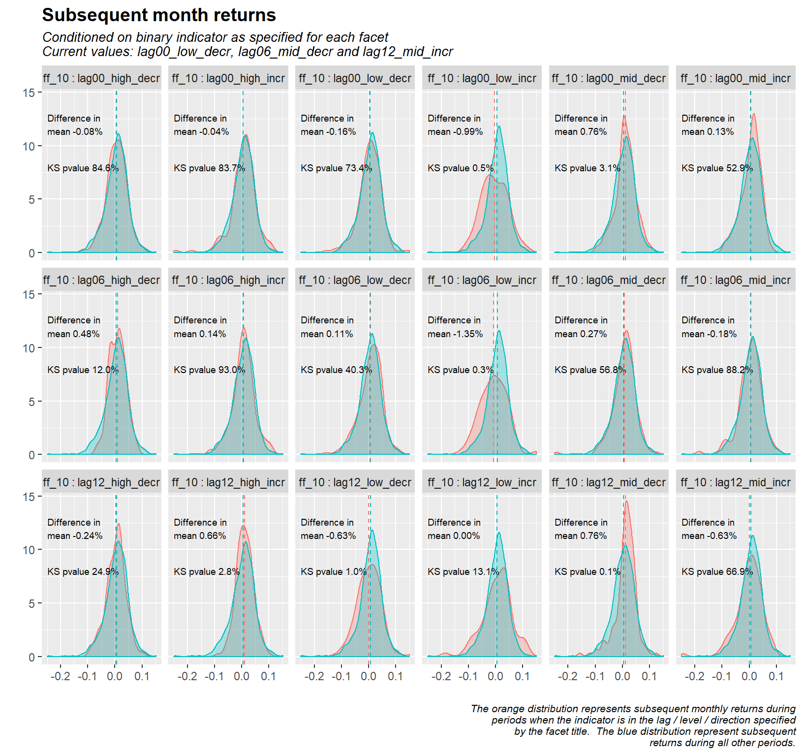
Finally, the following code plots the S&P 500 index and the yield curve and superimposes periods in which the maximum drawdown is more than 20% or the return is less than 2.5% over the following 6 months.
# plot S&P500 and market in/out shading
x11<-ggplot(data = x2,
aes(x = date,
y = close,
group = 1)) +
geom_line() +
scale_y_log10() +
geom_rect(data = sp_shade,
inherit.aes = FALSE,
aes(xmin = start, xmax = end, ymin = 0, ymax = Inf),
fill ='lightblue', alpha=0.5) +
theme_minimal() +
labs(title = "S&P 500 index",
subtitle = "log scale",
caption = "",
x = "Year",
y = "Close") +
geom_hline(yintercept = 0, color = "black") +
theme(plot.title = element_text(face = "bold", size = 14),
plot.subtitle = element_text(face = "italic", size = 9),
plot.caption = element_text(hjust = 0),
axis.title.y = element_text(face = "italic", size = 9),
axis.title.x = element_text(face = "italic", size = 9))
# Plot of selected yield curve & in/out shading
x12<-ggplot(data = x2,
aes(x = date,
y = ff_10,
group = 1)) +
geom_line() +
geom_rect(data = sp_shade,
inherit.aes = FALSE,
aes(xmin = start, xmax = end, ymin = -Inf, ymax = Inf),
fill = 'lightblue',
alpha = 0.5) +
geom_hline(yintercept = 0, color = "black") +
geom_hline(yintercept = quantile(x2$ff_10, probs = 0.33), color = "black", linetype = "dotted") +
geom_hline(yintercept = quantile(x2$ff_10, probs = 0.66), color = "black", linetype = "dotted") +
theme_minimal() +
labs(title = "",
subtitle = "",
x = "Year",
y = "Fed Funds, 10yr treasury spread",
caption = "Dashed lines represent upper and lower terciles.\nShading represents periods when the maximum drawdown is greater than\n20% or the return is less than 2.5% over the subsequent 6 monthly period.") +
theme(plot.title = element_text(face = "bold", size = 14),
plot.subtitle = element_text(face = "italic", size = 9),
plot.caption = element_text(face = "italic", size = 8),
axis.title.y = element_text(face = "italic", size = 9),
axis.title.x = element_text(face = "italic", size = 9))
# combine plots
plot_grid(x11, x12, ncol = 1, align = 'v')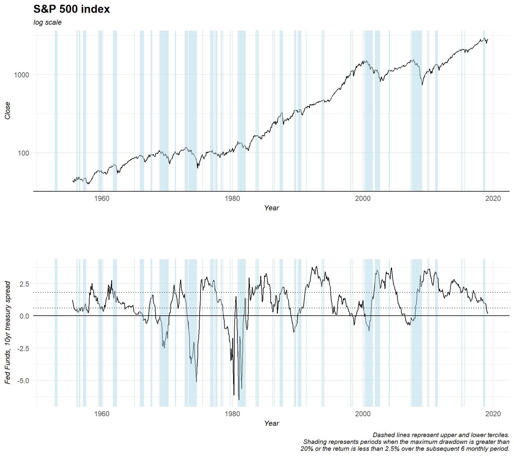 So, what do these plots tell us about the yield curve? Does the yield curve forecast the returns of the stock market?
Based on the histogram results, if the current value of the yield curve (defined as the Fed fund rate minus the 10-year Treasury rate) is low and rising (the facet called “lag00_low_incr”), we want to stay out of the market, the average of subsequent months returns are almost 1% lower than in all other periods. We are confident that this is a significant difference based on the results of the Kolmogorov Smirnov test, this test yields a p-value of 0.6% (the null hypothesis that the two samples were taken from the same distribution is rejected if the p-value is lower than your significance level - typically set to 5%).
If we look at the yield curve plot, we can confirm this visually. For example, it seems that the drawdowns in 2000 and 2008 are preceded by an increase in the yield curve from a low level. The second most significant bin for the current value of the yield curve is that when the level is in the mid tercile and the change is decreasing, the subsequent returns are 0.75% higher with a K-S p value of 3.7%. By way of comparison, the average monthly returns over the period under review are 0.61%.
Looking at lagged values of the yield curve, there are four situations that would lead us to take a view on the market:
1. When the 6-month lagged yield curve is low and increasing (lower subsequent returns)
2. When the 12-month lagged yield curve is high and increasing (higher subsequent returns)
3. When the 12-month lagged yield curve is low and decreasing (lower subsequent returns)
4. When the 12-month lagged yield curve is mid and decreasing (higher subsequent returns)
Limitations
Every analytical technique has its advantages and disadvantages. Discretisation or binning is useful in that it identifies nonlinearities, removes outliers, and is easy to interpret. However, the approach used above has some drawbacks. One drawback is that by design it peaks into the future. The measurement of tercile barriers in the 1970’s, for example, uses data from the 2000’s. A more robust approach would be to use a rolling starting point window to estimate the terciles for binning.
In addition, it may be that tercile bins are not suitable cut-offs, perhaps the traditional inversion of the yield curve or another level is an appropriate cut-off. We have not investigated this in the current analysis. Despite these limitations, this approach provides a high-level overview of the relationship between the level of the yield curve and subsequent stock market returns. This information can be useful to create more complex models, for example, to inform relevant dummy variables in a regression model.
The above code that generates the histogram and the line plots will of course be useful when analysing other time series, to that end they have been written into a function, the trans.plot() functions detailed here.