I recently finished reading Statistical Rethinking by Richard McElreath. The reviews are true, it’s a great book. As a bonus, it comes with 20 hours of supporting lectures taking you through the content.
Statistical Rethinking is an introduction to statistical modelling using Bayesian methods. Bayesian methods seem pretty popular at the moment, so whats the deal? To distill it into a couple of lines, Bayesian methods provide a distribution for model parameters and allow for incorporation of prior knowledge. This contrasts with frequentist methods which produce parameter point estimates and are limited to learning from data alone. The distribution of parameter values is called the posterior distribution and this represents the relative plausibility of different parameter values, conditional on the data and model. Having a posterior distribution comes in handy for expressing uncertainty in inference or prediction.
As stated in the preface, the book takes the philosophy that you will understand something better if you can see it working and implemented in code (preferably by yourself). The first method Statistical Rethinking introduces for computing a models posterior distribution is grid approximation. Grid approximation is one method of using the prior, the likelihood and data to estimate the posterior by applying Bayes’ theorem. In this post, I’m going to apply the books philosophy and calculate the posterior of human height data, manually, using grid approximation. In so doing, I will also need an estimation of the likelihood, and we will look into a couple of different ways to do this. The work on likelihood will use mock data.
Intuition comes when you look at problems from different angles. The concept of the likelihood has been a struggle, so fleshing it out multiple ways will help.
Overall, the purpose of this post is to convince myself that I have a decent grasp of how all this stuff works.
Grid approximation
“We can achieve an excellent approximation of the continuous posterior distribution by considering only a finite grid of parameter values. At any particular value of a parameter, p, it is simply a matter to compute the posterior probability: just multiply the prior probability OF p by the likelihood AT p, repeating this procedure for each value in the grid1.”
Data
We will start off fitting a normal distribution to data provided in the Rethinking R package. The Rethinking package accompanies the Statistical Rethinking text and is principally a teaching tool. As such it enforces an extended syntax. The idea being that exposing all modelling choices forces users to think about the modelling process in detail, encouraging an understand of what is going on “under the hood”. The package also includes a number of data sets.
The data in question is heights of a population under study. Fitting a normal distribution is equivalent to fitting a linear regression model that contains only an intercept.
This is a essentially a re-performance of code block 4.16 from the text. I’m not the first to look at this. See here, here, and here.
This is what the data looks like.
# Required packages
library(rethinking)

# Data
data(Howell1)
d <- Howell1
d2 <- d[d$age >= 18, ]

# Plot using rethinking function
plot(density(d2$height), main = 'Height data (cm)')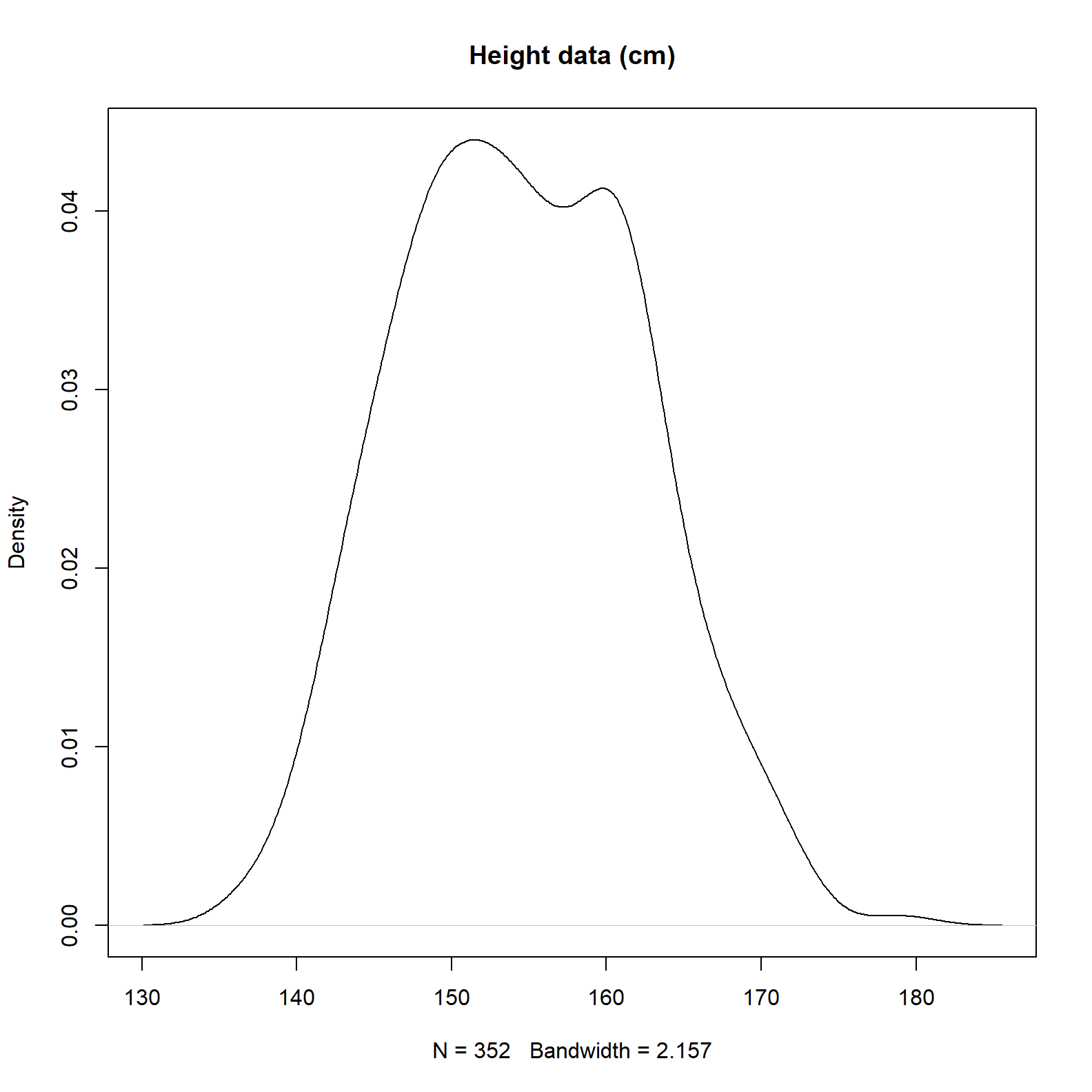
We can see there are 352 records and the average is somewhere near 155 centimeters.
Likelihood
The text book definition of the likelihood is the “probability of the data given a parameter value”. There are many other ways to get the concept across. The explanation that gels most with me is:
“the relative plausibility of the data, conditional on a parameter value”.
That comes from McElreath, as does,
“a likelihood is a prior for the data”, and “the likelihood is the relative number of ways that a parameter can produce the data”.
I think I can reconcile those three. Here is another soundbite type definition,
“the conditional distribution of the data given the parameters”, from the same source “this is called a likelihood because for a given pair of data and parameters it registers how ‘likely’ is the data”.2
As stated, I struggled grasping this concept. Code will help.
Before attacking the problem with the data mentioned above, lets work through an extremely simple example.
An intuitive example of likelihood
The very simple example below should help fleshing out the quoted definitions in the paragraph above.
First we take some data and estimate the mean and standard deviation.
# Some data
dat <- c(148, 149, 150, 151, 152)

# The mean and standard deviation (150 & 1.58) thereof
c(mean(dat), sd(dat))
## [1] 150.000000 1.581139We create a data frame containing this data, and include columns for a mean and standard deviation. Three repeats of the 5 records are made. The first, labelled “A”, correspond to the population mean and standard deviation (150 and 1.58), the next two, labelled “B” and “C”, have a mean and standard deviation that is slightly different. We will use the columns containing the difference mean and standard deviation to calculate the log-likelihood3.
df <- data.frame(
  param_set = rep(c('A','B','C'), each = 5),
  mu = c(rep(150,10), rep(160,5)),
  sigma = c(rep(1.6, 5), rep(7, 5), rep(1.6, 5)),
  data = rep(dat, 3)
  )
Now to calculate the log-likelihood and view the results.
# Calculate the log-likelihood for each data point
df$log_lik <- sapply(df[,2:4], dnorm, x = df$dat, mean = df$mu, sd = df$sigma)[,1]
df$log_lik <- round(df$log_lik,3)

# View
library(DT)
datatable(df, options = list(autoWidth = FALSE, searching = FALSE))# %>% format('log_lik', 1)
Finally we sum the log-likelihood for each set of mean and standard deviation provided.
aggregate(. ~ param_set, data = df[,c('param_set', 'log_lik')], sum)## param_set log_lik
## 1 A -8.897
## 2 B -14.427
## 3 C -106.554Leaning on our definition above, the three values returned represents the relative plausibility of seeing the data assuming the parameters. The maximum log-likelihood belongs to parameter set A. This is of course as expected, the first example has the exact same parameters as the underlying data. The data is more ‘likely’ to arise with these parameters.
What we have done here is measure the ways parameters can produce the data. We have assumed the data comes from a specific distribution (normal in this case), and compared the expected value for different sets of parameters. The dnorm function allows us to perform this comparison and is explained in more detail below.
Note that the exercise above can be replicated in an excel spreadsheet quite easily. The NORM.DIST and LN functions can be used to calculate the log-likelihood.
We can also perform this in a more succinct manner as shown below. Identical to the previous example, we calculate log-likelihood, firstly using the exact mean and standard deviation, then with differing mean and standard deviation for the same data set.
ll_a <- sum(dnorm(x = dat, mean = 150, sd = 1.6, log = TRUE))   # same parameters
ll_b <- sum(dnorm(x = dat, mean = 150, sd = 10, log = TRUE))    # different parameters
ll_c <- sum(dnorm(x = dat, mean = 160, sd = 1.6, log = TRUE))   # different parameters

c(ll_a, ll_b, ll_c)
## [1] -8.897836 -16.157618 -106.554086Again, the three values returned represents the relative plausibility of seeing the data assuming the parameters.
OK, back to the data set at hand. Below we perform grid approximation proper.
Log-likelihood - step 1
Referencing the grid approximation definition I first quoted above, we create a data structure for the "at any particular value of a parameter, p" component. We create a grid for combinations of means and standard deviations for which the likelihood is calculated over. The code below cross joins 100 mu’s and 100 sigmas for 10,000 distinct combinations. These are the parameters we are trying to calculate a posterior distribution over.
mu_list <- seq(from = 140, to = 170, length.out = 100)
sigma_list <- seq(from = 7, to = 9, length.out = 100)
post <- expand.grid(mu = mu_list, sigma = sigma_list)
Log-likelihood - step 2
For each of the 10,000 combinations of mu and sigma, calculate the sum of the probability density function for each of 352 values of height. This is the “likelihood at p” component.
We will use the function dnorm to do this. Before getting into the details, it is a good idea to take note of what exactly dnorm is doing.
The function dnorm returns the value of the probability density function (“pdf”) for the normal distribution given some data and values for the mean (mu), and standard deviation (sigma). dnorm will give us the “height” of the pdf of the normal distribution at whatever value of data (x) we provide. The height of the pdf represents the relative probability of getting the value of x assuming the data is normally distributed, and also assuming the mu and sigma parameters supplied.4
Again, referencing the definition of grid approximation above, the code below calculates the “likelihood AT p” component. For exposition purposes, we will do this in both a vectorised and looped manner.
# Vectorised using sapply
post$ll <- sapply(
  X = 1:nrow(post),
  FUN = function(i) sum(dnorm(x = d2$height, mean = post$mu[i], sd = post$sigma[i], log = TRUE))
)

# Repeating the above sapply construction of log-likelihood, using a for loop
ll_via_loop <- vector(mode = "double", length = nrow(post))
for (mu_sigma in 1:nrow(post)) {
  ll_height <- vector(mode = "double", length = nrow(d2))
  for (height in 1:nrow(d2)) {
    ll_height[height] <- dnorm(x = d2$height[height], mean = post$mu[mu_sigma], sd = post$sigma[mu_sigma], log = TRUE)
  }
  ll_via_loop[mu_sigma] = sum(ll_height)
}

# Assign to df
post$ll2 <- ll_via_loop

# Check we are returning the same results
sum(abs(post$ll - post$ll2))
## [1] 0Good, we now have a likelihood. It look like this.
image_xyz(post$mu, post$sigma, post$ll, col =gray.colors(25, start = 0.1, end = 0.9, rev = TRUE), xlab = "mean", ylab = "standard deviation")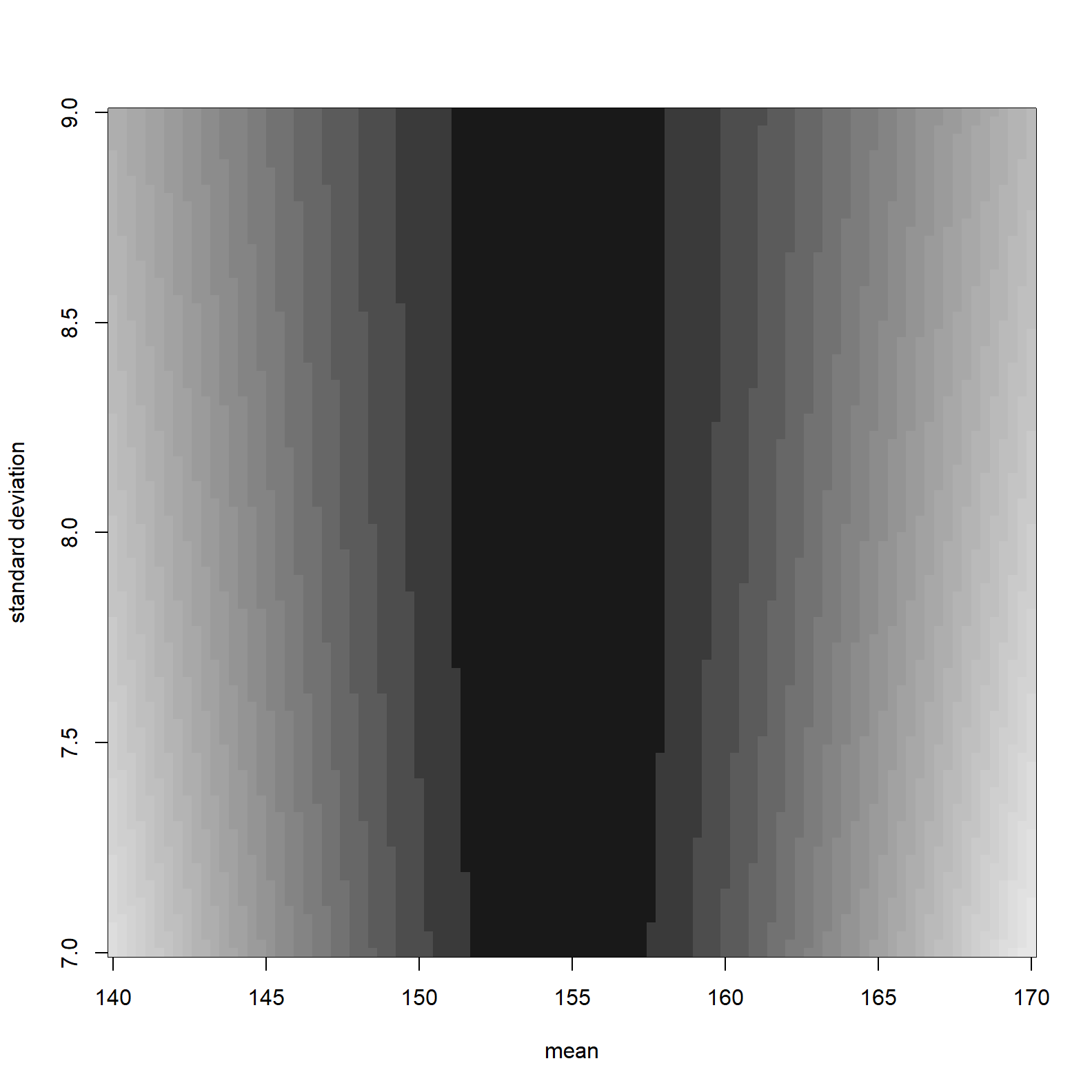
The darker shading represents higher log-likelihoods. The maximum log likelihood is:
post[which.max(post$ll), c("mu", "sigma", "ll")]## mu sigma ll
## 3649 154.5455 7.727273 -1219.413Prior
The prior in a modelling context is the “probability of a parameter value”. A prior embodies our knowledge before seeing any data, or to put it another way, represents the prior plausibility of a parameter value. For the problem at hand, we will select a mean of 178cm and standard deviation of 20cm. 178cm is the average male height and we will imagine we have not seen the particular data set presented above. A standard deviation of 20 assumes 2/3 of the population will be between 158cm and 198cm and 95% between 138cm and 218cm. That seems very broad and as such would be considered a weak prior. It does not encode a strong assumption as a specific prior plausibility.
Compute the product of likelihood and priors
This is the numerator of Bayes’ theorem. We add as opposed to multiply these since we are using logs. This gives us the unstandardised posterior.
The comments in the code below show how our prior is accounted for.
post$prod <-
  post$ll +                                                 # log-likelihood per above
  dnorm(x = post$mu, mean = 178, sd = 20, log = TRUE) +     # prior for mean (normal)
  dunif(x = post$sigma, min = 0, max = 50, log = TRUE)      # prior for standard deviation (uniform)
We now have an unstandardised posterior, this is scaled with the code below to produce a posterior probability. Note that the code below adds the line given in this post, ensuring the posterior sums to one.
post$prob <- exp(post$prod - max(post$prod))
post$prob <- post$prob/sum(post$prob)
Lets look at the parameters associated with the maximum posterior probability.
post[which.max(post$prob), c("mu", "sigma", "ll", "prob")]## mu sigma ll prob
## 3649 154.5455 7.727273 -1219.413 0.007992941It is worth noting that the parameters associated with the maximum likelihood and the maximum posterior probability are identical. That won’t always be the case. In this case it indicates that the data has overwhelmed the relatively weekly informative prior.
Here is a plot of the posterior distribution.
#contour_xyz(post$mu, post$sigma, post$prob)
image_xyz(post$mu, post$sigma, post$prob, col = gray.colors(25, start = 0.1, end = 0.9, rev = TRUE), xlab = "mean", ylab = "standard deviation", xlim = c(150,160), ylim= c(7,8.5))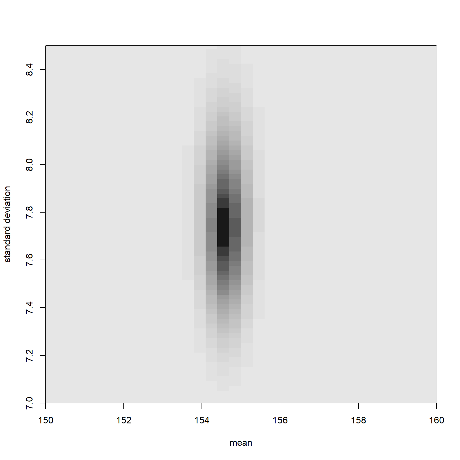
The parameter values associated with higher posterior probability are much more focused than parameter values associated with high likelihoods. This is because of the impact of the prior. Parameters with low prior probability have been down weighted.
An alternate derivation of the log-likelihood
I mentioned I was going to look at this from a couple of different perspectives.
This stack overflow answer explaining Maximum Likelihood Estimation provides another angle to looking at the likelihood. This example calculates the likelihood using a function, and then optimises the parameters of that function to maximise the log-likelihood. The author has created a grid, not for the purpose of posterior estimation, but rather as a demonstration tool for the optimisation performed.
I’m going to use the log-likelihood grid created using this alternate method to estimate a posterior, and then use the method applied above to hopefully arrive at the same result.
In this case we have two parameters to estimate, an intercept and slope of a linear model.
To start we create some mock data. The parameters to retrieve are alpha and beta, the intercept and slope of the linear model.
set.seed(123)
n <- 200
alpha <- 9
beta <- 2
sigma <- 0.8
theta = c(alpha, beta, sigma)
data <- data.frame(x = runif(n, 1, 10))
data$y <- alpha + beta*data$x + rnorm(n, 0, sigma)

plot(data$x, data$y)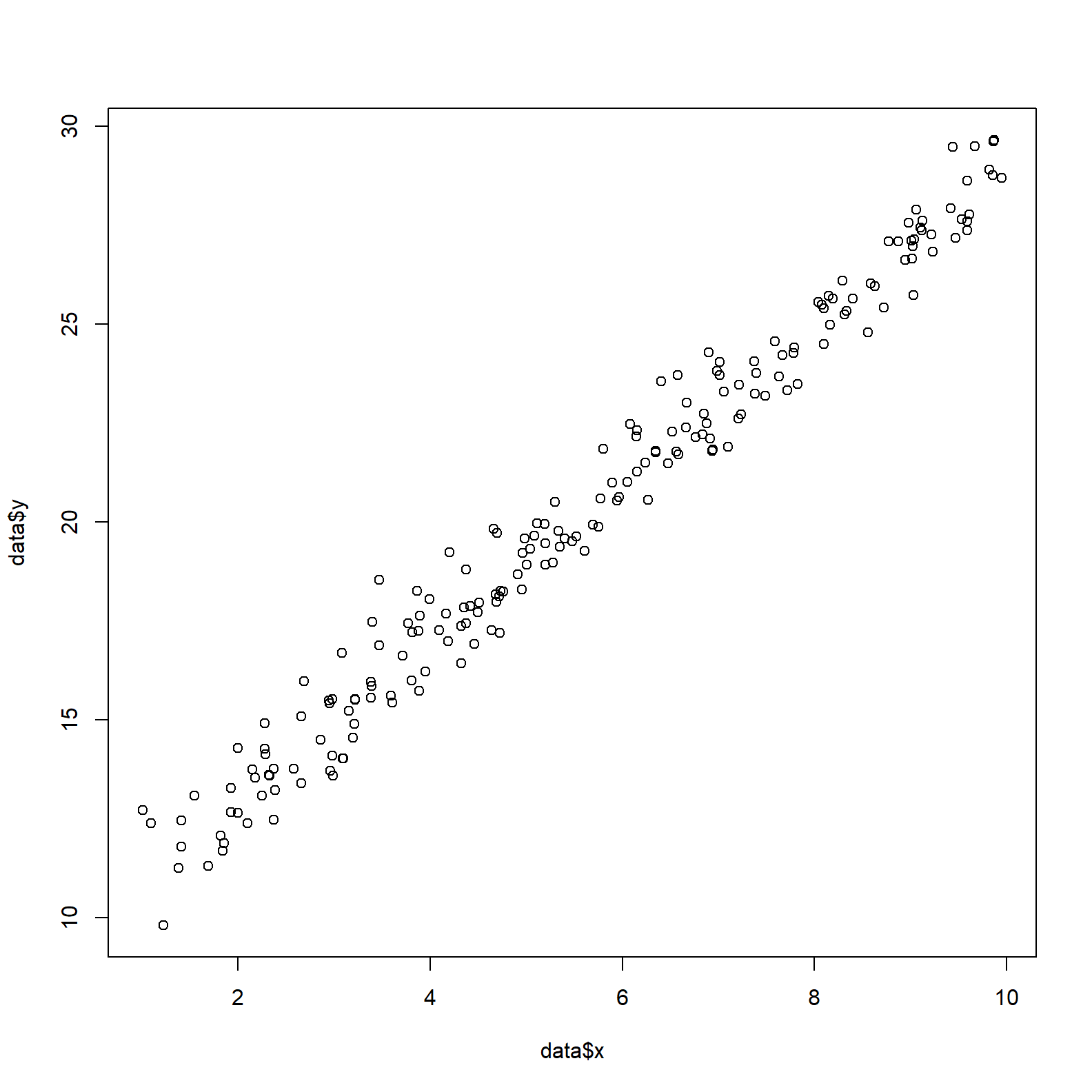
The log-likelihood function.
linear.lik <- function(theta, y, X){
  n      <- nrow(X)
  k      <- ncol(X)
  beta   <- theta[1:k]
  sigma2 <- theta[k+1]^2
  e      <- y - X%*%beta
  logl   <- -.5*n*log(2*pi)-.5*n*log(sigma2)-((t(e) %*% e)/(2*sigma2))
  return(-logl)
}
Note that the line of code defining the “logl” above (the value returned by the function) is performing the same function as dnorm in the grid approximation method. It is estimating the “likelihood at p”.
Next, the log-likelihood function is applied to the parameter values. The code below is similar to the grid approximation method. In this case the grid is created on the fly with nested for loops.
surface <- list()
k <- 0
for(alpha in seq(8, 10, 0.1)){
  for(beta in seq(0, 3, 0.1)){
    for(sigma in seq(0.1, 2, 0.1)){
      k <- k + 1
      logL <- linear.lik(theta = c(alpha, beta, sigma), y = data$y, X = cbind(1, data$x))
      surface[[k]] <- data.frame(alpha = alpha, beta = beta, sigma = sigma, logL = -logL)
    }
  }
}
Now we find the maximum of the log-likelihood (the MLE) using R’s optimisation function optim.
linear.MLE <- optim(
  fn=linear.lik,
  par=c(1,1,1),
  lower = c(-Inf, -Inf, 1e-8),
  upper = c(Inf, Inf, Inf),
  hessian=TRUE,
  y=data$y,
  X=cbind(1, data$x),
  method = "L-BFGS-B"
  )

linear.MLE$par
## [1] 9.0742422 1.9875715 0.7677577The first two numbers represent maximum likelihood estimates of the alpha and beta parameters. The third is sigma. With this we have successfully retrieved the parameters values invoked when mocking up the data.
Let’s estimate the parameters using a couple of different methods.
Parameters associated with the maximum log-likelihood via interrogation of the surface grid (this is equivalent to the grid used in grid approximation).
surfacedf <- data.frame(do.call(rbind, surface))
surfacedf[which.max(surfacedf$logL), ]
## alpha beta sigma logL
## 6608 9 2 0.8 -231.4109These by definition have to be one of the entries in the grid, and so are slightly different to that obtained via the optimisation of the log-likelhood function.
Here is the parameter estimation using ordinary least squares via base R’s lm function.
lm(y ~ x, data = data)##
## Call:
## lm(formula = y ~ x, data = data)
##
## Coefficients:
## (Intercept) x
## 9.074 1.988And finally the true parameters.
theta## [1] 9.0 2.0 0.8Similar to the height data, we can plot the log-likelihood over the grid range chosen as so.
surfacedf_mean <- aggregate(logL ~ alpha + beta, data = surfacedf[,c('alpha', 'beta', 'logL')], sum)
image_xyz(surfacedf_mean$alpha, surfacedf_mean$beta, surfacedf_mean$logL, col = gray.colors(100, start = 0.1, rev = TRUE), xlab = "alpha", ylab = "beta")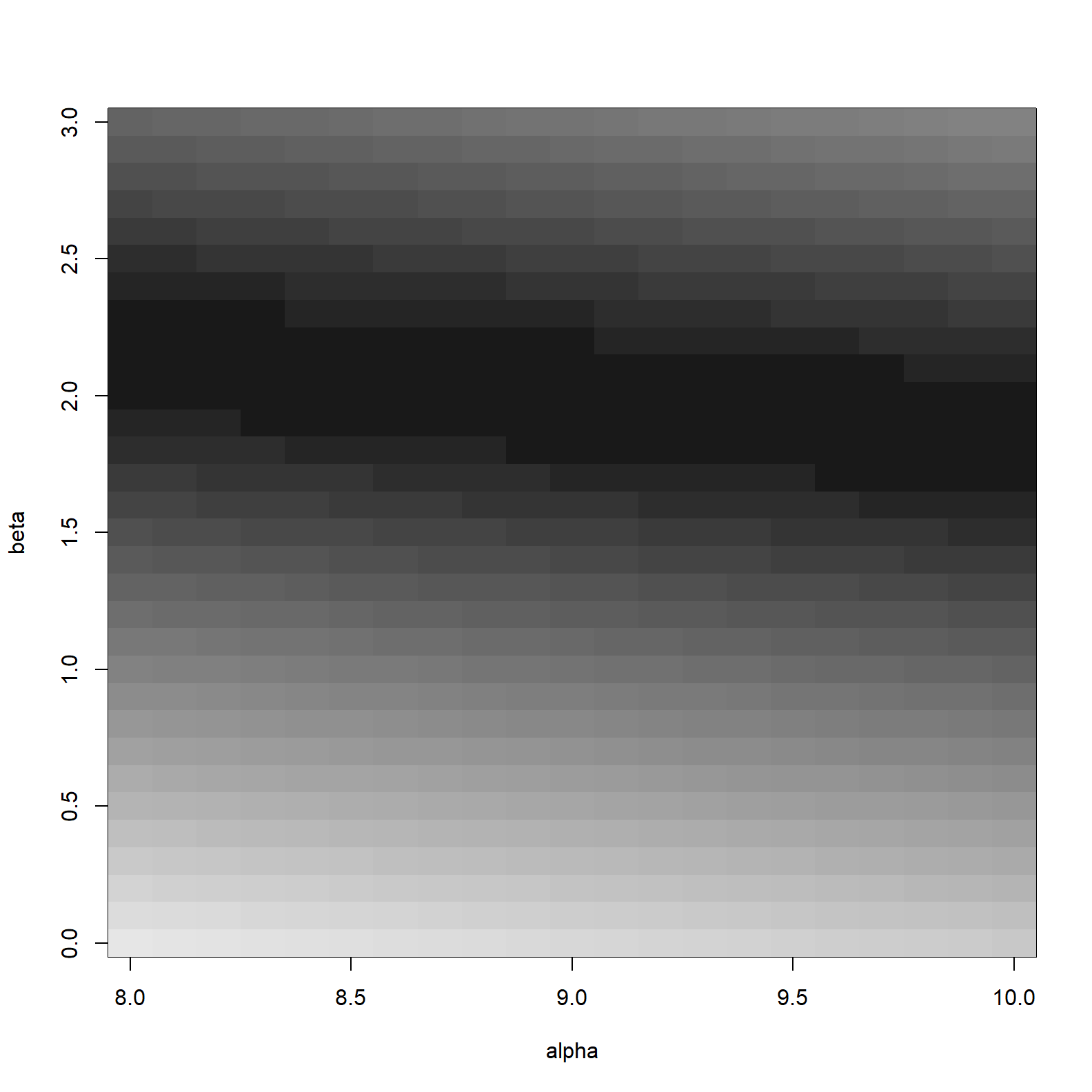
Grid approximation
Returning to grid approximation. Below we estimate parameters using the original grid approximation method.
# Grid - we will use the 'surface' data frame created above
post2 <- surfacedf

# Log-likelihood
post2$ll <- sapply(
  X = 1:nrow(post2),
  FUN = function(i) sum(dnorm(
    x    = data$y,                                   # Note that it is the dependent variable here
    mean = post2$alpha[i] + (post2$beta[i] * data$x),
    sd   = post2$sigma[i],
    log  = TRUE
  ))
)


# Posterior
post2$prod1 <-
  post2$ll +                                                # log-likelihood per above
  dnorm(x = post2$alpha , mean = 0, sd = 5, log = TRUE) +   # prior for alpha
  dnorm(x = post2$beta  , mean = 0, sd = 5, log = TRUE) +   # prior for beta
  dexp(x = post2$sigma , rate = 1, log = TRUE)              # prior for standard deviation


# Relative posterior probability
post2$prob1 <- exp(post2$prod1 - max(post2$prod1))
post2$prob1 <- post2$prob1/sum(post2$prob1)


# MLE
post2[which.max(post2$ll), c("alpha", "beta", "sigma", "logL", "ll")]
## alpha beta sigma logL ll
## 6608 9 2 0.8 -231.4109 -231.4109As expected, everything agrees.
Rethinking package
As mentioned above, the Rethinking R package accompanies the Statistical Rethinking text and is principally a teaching tool. Rethinking includes a function called quap. This function performs a quadratic approximation to find the posterior distribution. To quote directly from the text.
“Under quite general conditions, the region near the peak of the posterior distribution will be nearly Gaussian-or”normal“-in shape. This means the posterior distribution can be usefully approximated by a Gaussian distribution. A Gaussian distribution is convenient, because it can be completely described by only two numbers: the location of its center (mean) and its spread (variance).
A Gaussian approximation is called”quadratic approximation" because the logarithm of a Gaussian distribution forms a parabola. And a parabola is a quadratic function. So this approximation essentially represents any log-posterior with a parabola."5
Below, parameters are estimated using quadratic approximation via quap.
reth_mdl <- quap(
  alist(
    y ~ dnorm(mu, sigma),
    mu <- alpha + beta * x,
    alpha ~ dnorm(0, 5),
    beta ~ dnorm(0, 5),
    sigma ~ dexp(1)
  ) , data = data)

precis(reth_mdl)
## mean sd 5.5% 94.5%
## alpha 9.0679471 0.13382486 8.8540691 9.2818251
## beta 1.9885120 0.02202053 1.9533190 2.0237051
## sigma 0.7662957 0.03820537 0.7052362 0.8273553Once again, our parameters estimates are in agreement.6
Finally, lets see if we can replicate the compatability intervals returned by quap above (the last two columns). To do this we will manually extract samples from the posterior distribution derived via grid approximation. The code below borrows from p. 55 - sections 3.3 & 3.10, and p. 85 - section 4.19 of the Statistical Rethinking text.
sample_rows <- sample(1:nrow(post2), size = 1e4, replace = TRUE, prob = post2$prob1)
sample_alpha <- post2$alpha[sample_rows]
sample_beta <- post2$beta[sample_rows]
sample_sigma <- post2$sigma[sample_rows]

c('alpha', quantile(sample_alpha, c(0.055, 0.945)))
## 5.5% 94.5%
## "alpha" "8.9" "9.1"c('beta', quantile(sample_beta, c(0.055, 0.945)))## 5.5% 94.5%
## "beta" "2" "2"c('sigma', quantile(sample_sigma, c(0.055, 0.945)))## 5.5% 94.5%
## "sigma" "0.7" "0.8"These estimates match up reasonably well. Some values are slightly different and that is due to our grid not being granular enough to capture the variation in the continuous results returned by quadratic approximation.
Conclusion
With this post my aim has been to document my thoughts and learning in relation to the intuition of bayesian inference. A big part of this learning process is the concept of the likelihood. This is definitely the hardest concept to grasp and is also the most computationally intense. As such it has been covered in detail, going back to first principles.
I think I now have, to quote myself, “a decent grasp of how all this stuff works”. In addition, the analysis above will serve as a nice reference point going forward.
References
https://xcelab.net/rm/statistical-rethinking/
https://en.wikipedia.org/wiki/Bayes%27_theorem
https://github.com/rmcelreath/rethinking
https://poissonisfish.com/2019/05/01/bayesian-models-in-r/
https://rileyking.netlify.app/post/bayesian-modeling-of-censored-and-uncensored-fatigue-data-in-r/
https://allendowney.github.io/ThinkBayes2/hospital.html
https://www.psychologicalscience.org/observer/bayes-for-beginners-probability-and-likelihood
https://www.image.ucar.edu/pub/TOY07.4/nychka2a.pdf
https://rpsychologist.com/likelihood/
https://stats.stackexchange.com/questions/112451/maximum-likelihood-estimation-mle-in-layman-terms
https://www.uio.no/studier/emner/matnat/math/STK4180/v16/clp_oct2015_pages1to205.pdf
https://seankross.com/notes/dpqr/
https://stats.stackexchange.com/questions/371491/understanding-bayesian-model-code-from-chapter-4-of-statistical-rethinking
McElreath p40.↩︎
Log-likelihood because using logs we can sum instead of taking the product (that’s just convenient). Also, logs work better when dealing with very small numbers, as is the case with likelihoods and priors.↩︎
This site is a good reference, and forms the basis for this paragraph.↩︎
McElreath p42.↩︎
Note that calling the `
quapfunction more than once in the same session can result in vastly different results. I will have to dive into the documentation to understand this.↩︎